Background

The challenge with missing population data is not unique to humanitarian settings alone prompting research interest into the use of alternative data sources to fill in the gap for missing census records. With the growing availability of high-resolution satellite imagery coupled with recent advances in machine learning methods, organizations like WorldPop, Facebook, and the EU’s JRC, to name a few, have been able to produce extremely detailed population estimates for all countries across the globe. Those estimates are provided in the form of a fine grid overlaid on top of the target geographic area where the grid cells contain estimates of the population in each cell hence the name “gridded population data”.

The idea of geospatial sampling is to use this kind of gridded population data to fill in for the missing sampling frame. While population grids may not be 100% perfect, independent verifications have found them to be surprisingly accurate and they are definitely a step-up from not having household surveys or the use of non-probabilistic sampling methods.

We’re going to use Syria as an example in this tutorial. A war-torn country where the official population figure of 26.5 million widely diverges from the UN Population Division’s 17.5 million estimate making it difficult to rely on official data for sampling purposes.

Let’s first load up the necessary packages.

## This function will retrieve the packae if they are not yet installed.
using <- function(...) {
    libs <- unlist(list(...))
    req <- unlist(lapply(libs,require,character.only = TRUE))
    need <- libs[req == FALSE]
    if (length(need) > 0) { 
        install.packages(need)
        lapply(need,require,character.only = TRUE)
    }
}

## Getting all necessary package
using("tidyverse", "osmdata", "ggmap", "OpenStreetMap", "viridis", "stars", "sf")

rm(using)

Next we’ll import WorldPop’s 2020 UNPD-adjusted Syria population grid with a cell resolution of 3 arc seconds (approx. 100 meters at the equator).

# url <- "ftp://ftp.worldpop.org.uk/GIS/Population/Global_2000_2020/2020/SYR/syr_ppp_2020_UNadj.tif"

#ppp100m <- read_stars(url) %>% select(ppp = 1) # ppp stands for "population per pixel"
file <- paste0(getwd(),"/syr_ppp_2020_UNadj.tif")
ppp100m <- read_stars(file) %>% select(ppp = 1) 

To pull in some satellite imagery for illustration purposes, there’s 2 options:

• Google Maps API with ggmap package. User shall first enabled billing on your own account in order to create their API key

• Bing imagery using the OpenStreetMap package (no account required).

to keep it simpler, the rest of the tutorial will use the second option.

#key <- Sys.getenv("GMAPS_API_KEY") # Need to have this configured in .Rprofile first
# as of mid-2018, registering with Google Cloud to obtain an API key is required to use any of Google's services, including get_googlemap. Usage and billing may apply
## do not forget to enable the static maps API on google cloud to avoid message such as 
# "The Google Maps Platform server rejected your request. This API project is not authorized to use this API."
## This will require you to first enabled billing on your own account
#register_google(key)

Delineating Populated Places

If gridded population data can substitute for missing census records, what about the problem of missing human settlement maps?

Luckily, a recent proposal endorsed by the UN Statistical Commission’s 51st session allows for the delineation of cities, urban, and rural areas using gridded population data without the need for administrative boundary maps.

The Degree of Urbanization method, as it is known, starts with a population grid of 1 km^2 cells which are then clustered based on population density, contiguity, and population size to identify human settlement boundaries. The classification of grid cells/clusters is summarized in the following table:

douclass <- 
  tribble(
    ~"Class", ~"Population/km^2", ~"Total Population", ~"Human Settlement", ~"Common Name",
    "Urban center", ">= 1,500", ">= 50,000", TRUE, "City",
    "Dense urban cluster", ">= 1,500", "5,000 - 49,999", TRUE, "Dense Town",
    "Semi-dense urban cluster", ">= 300", ">= 5,000", TRUE, "Semi-dense Town",
    "Suburban or peri-urban cells", ">= 300", NA, FALSE, "Suburban or peri-urban area",
    "Rural cluser", ">= 300", "500 - 4,999", TRUE, "Village",
    "Low density rural grid cells", ">= 50", NA, FALSE, "Dispersed rural area",
    "Very low density rural grid cells", "< 50", NA, FALSE, "Mostly uninhabited areas")

douclass %>% rmarkdown::paged_table()

Do note that the use of “common name” here is somewhat misleading. According to the classification, an administrative unit should be designated as a city, for example, if the majority of its population resides in urban centers but the two are not meant to be synonymous. The distinction, however, is immaterial for our purposes because our objective is to identify populated places not to recover the exact (often arbitrary) boundaries of administrative units.

Moving on, operationalizing the definition necessitates aggregating every 10x10 cells in our 100m x 100m population grid into a “supercell” of 1 km^2 each.

# FIXME: the original raster is only 100m at the equator. That's about 85m in Syria because of Earth's curvature.
# Need to reflect that below.
ppp1km <-
  st_as_stars(
    st_bbox(ppp100m),
    dx = st_dimensions(ppp100m)$x$delta*10,
    dy = st_dimensions(ppp100m)$y$delta*10) %>%
  st_warp(
    src = ppp100m,
    method = "average",
    use_gdal = TRUE)

ppp1km <- ppp1km %>% select(ppp = 1) %>% mutate(ppp = ppp*100)

N.B.: This calculation actually under-estimates the population within 1km from the border because of the way method="average" weighs NODATA cells in the src raster. This should be fixed with the upcoming release of GDAL 3.1 which introduces method="sum" to handle similar use cases.

Here’s what our gridded population map looks like.

ggplot() + 
  geom_stars(data = ppp1km) +
  scale_x_continuous(labels = function(x) { str_c(x, "°", if_else(x >= 0, "E", "W")) }) +
  scale_y_continuous(labels = function(y) { str_c(y, "°", if_else(y >= 0, "N", "S")) }) +
  #scale_fill_viridis_b(
  scale_fill_viridis(option = "B",
    trans = "log10",
    breaks = 10^(0:3),
    label = scales::label_comma(accuracy = 1),
    direction = -1) +
  theme_minimal() +
  labs(
    title = "2020 Syria Population (UNPD-adjusted)",
    fill = "persons/km²",
    x = NULL, y = NULL)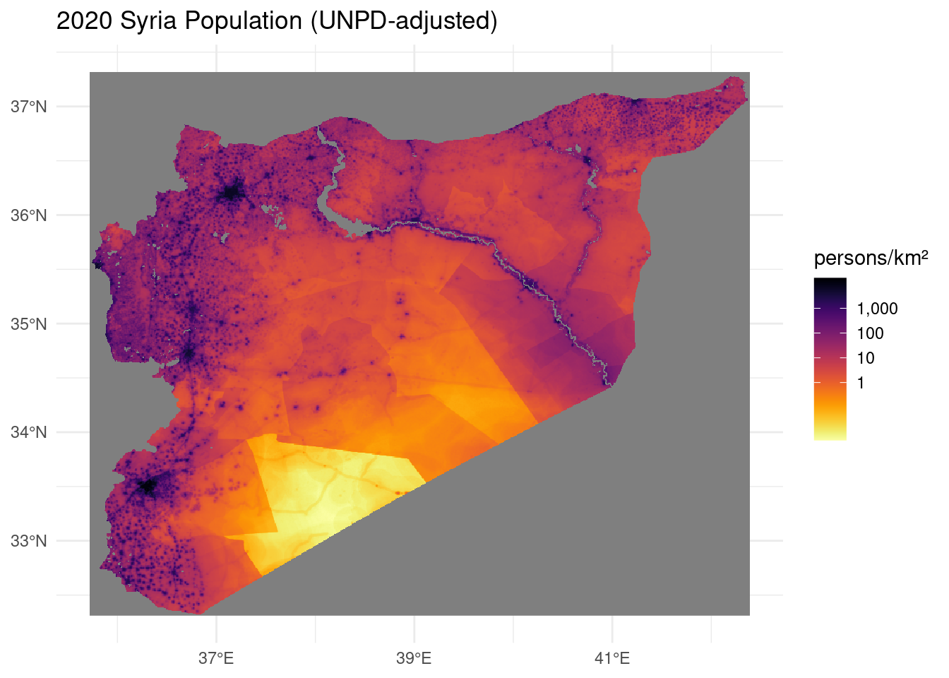

Now we can classify cells based on their Degree of Urbanization:

douclust <- function(data, type, cellmin, popmin) {
  data %>% 
    filter(ppp >= cellmin) %>% 
    mutate(
      cluster = 
        st_disjoint(., .) %>% as.dist() %>% hclust(method = "single") %>% cutree(h = 0)) %>% 
    group_by(cluster) %>% 
    summarize(class = type, pop = sum(ppp)) %>% 
    filter(pop >= popmin) %>% 
    select(-cluster)
}

ppp1km_sf <- ppp1km %>% st_as_sf()

workingset <- ppp1km_sf

rural_vlow <- 
  workingset %>% 
  filter(ppp < 50) %>% 
  summarize(class = "Very low density rural grid cells", pop = sum(ppp))

workingset <- workingset %>% filter(ppp >= 50)

urban_centers <- workingset %>% douclust("Urban center", 1500, 50000)

urban_clusters <- workingset %>% douclust("Urban cluster", 300, 5000)

workingset <- workingset %>% st_difference(st_union(urban_centers))

urban_dense_clusters <- workingset %>% douclust("Dense urban cluster", 1500, 5000)

workingset <- workingset %>% st_difference(st_union(urban_dense_clusters))

urban_semidense_clusters <- 
  workingset %>% 
  douclust("Semi-dense urban cluster", 300, 5000) %>% 
  st_filter(
    st_union(st_union(urban_centers), st_union(urban_dense_clusters)),
    .predicate = negate(st_is_within_distance),
    dist = units::set_units(2, km))

workingset <- workingset %>% st_difference(st_union(urban_semidense_clusters))

urban_suburban_cells <- 
  workingset %>% 
  st_filter(urban_clusters, .predicate = st_within) %>% 
  douclust("Suburban or peri-urban grid cells", 0, 0)

workingset <- workingset %>% st_difference(st_union(urban_suburban_cells))

rural_clusters <- workingset %>% douclust("Rural cluster", 300, 500)

workingset <- workingset %>% st_difference(st_union(rural_clusters))

rural_low <- workingset %>% summarize(class = "Low density rural grid cells", pop = sum(ppp))

rm(workingset)

doumap <- 
  rbind(
    urban_centers,
    urban_dense_clusters, urban_semidense_clusters, urban_suburban_cells,
    rural_clusters, rural_low, rural_vlow)

And here’s what our map looks like based on the Degree of Urbanization:

doumap %>% 
  ggplot() + 
  geom_sf(aes(fill = as_factor(class)), color = NA) +
  scale_x_continuous(labels = function(x) { str_c(x, "°", if_else(x >= 0, "E", "W")) }) +
  scale_y_continuous(labels = function(y) { str_c(y, "°", if_else(y >= 0, "N", "S")) }) +
  scale_fill_viridis_d() +
  theme_minimal() +
  labs(title = "Degree of Urbanization", fill = NULL)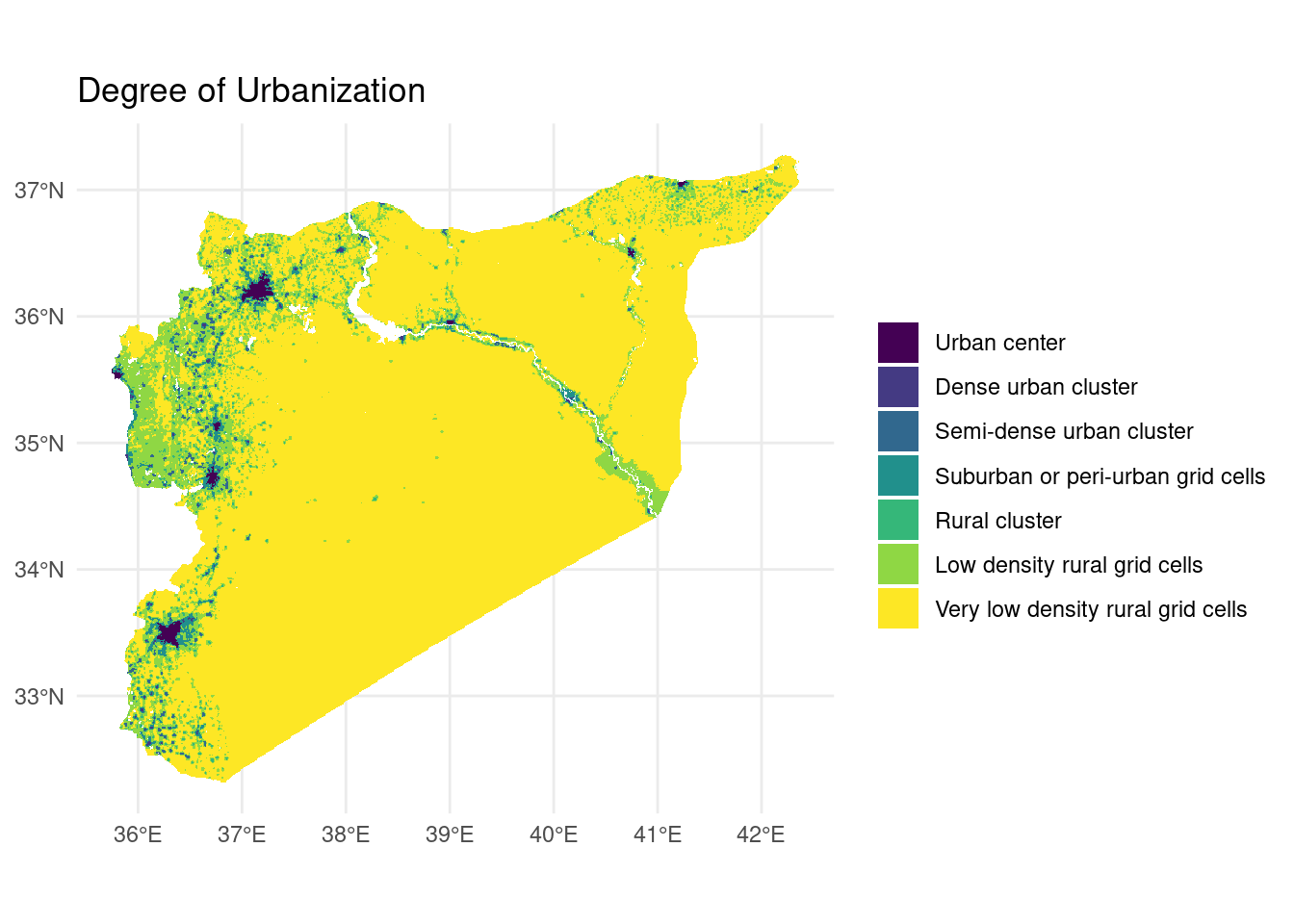

It may be difficult to see from the above map, but we’ve identified 8 cities, 185 towns, and 619 villages using this method. According to our mapping, 59% of the Syrian population lives in urban areas. Meantime, the World Bank puts the figure at 54%. Close enough. This suggests that the Degree of Urbanization method has correctly picked up all major populated places as expected and without the need for a pre-produced map of settlement boundaries.

Geospatial Sampling

Armed with our population grid and populated places map, we now have the necessary ingredients for multi-stage cluster sampling. The only difference with geospatial sampling is that, instead of using census enumeration areas as sampling units as we normally would, we’re going to use the 1km x 1km supercells and the 100m x 100m cells as primary and secondary sampling units, respectively. Sampling is done using probability proportional to size where the measure of size is cell population. A third stage of sampling is also required to select dwellings within the secondary sampling units, by randomly drawing a point in the cell and choosing the nearest building, followed by a fourth and final stage in the field to select respondent units from multi-household dwellings.

The beauty of R is that it allows us to do all this in just a few lines of code. Simple Features let us manipulate geodata no differently from any regular tabular dataset without the need for specialized GIS software. To illustrate how this works, let’s say we were planning a needs assessment in Aleppo with a target sample of 1,000 households spread over 100 clusters of 10 households each.

set.seed(1)

# Extract Aleppo knowing that it's the second largest city in Syria
aleppo <- urban_centers %>% arrange(desc(pop)) %>% slice(2)

nclust <- 100
hh_per_clust <- 10

s <- 
  ppp1km_sf %>% 
  st_filter(aleppo, .predice = st_within) %>% 
  mutate(psuid = row_number()) %>% 
  sample_n(nclust, weight = .$ppp) %>% 
  rename(psupop = ppp, psugeometry = geometry) %>% 
  rowwise() %>% 
  mutate(
    ssu = 
      ppp100m %>% 
      st_crop(psugeometry) %>% 
      st_as_sf() %>% 
      mutate(ssuid = row_number()) %>% 
      sample_n(hh_per_clust, weight = .$ppp) %>% 
      rename(ssupop = ppp, ssugeometry = geometry) %>% 
      list()) %>% 
  unnest(ssu) %>% 
  st_as_sf(sf_column_name = "ssugeometry") %>% 
  mutate(tsugeometry = st_sample(., rep(1, nrow(.))))

Or, for the more visually inclined, here’s what the primary sampling stage looks like:

# Draw a random PSU to use as an example
ex <- 
  s %>% filter(psuid == sample(psuid, 1, prob = psupop)) %>% st_set_geometry("psugeometry")

## Extract bounding box to get bing imagery
bbox <- aleppo %>%  st_bbox()

## Extract imagery background
map <- openmap(c(bbox$ymax,bbox$xmin), c(bbox$ymin,bbox$xmax), 
               zoom = 11,
               type =  "bing" ,
               mergeTiles = TRUE)



## OSM CRS :: "+proj=merc +a=6378137 +b=6378137 +lat_ts=0.0 +lon_0=0.0 +x_0=0.0 +y_0=0 +k=1.0 +units=m +nadgrids=@null +no_defs"
map.latlon <- openproj(map, projection = "+proj=longlat +ellps=WGS84 +datum=WGS84 +no_defs")

psubg <- 
  
## option for google map background---   
#   get_googlemap(
#     center = aleppo %>% st_centroid() %>% st_coordinates(),
#     zoom = 11,
#     scale = 1,
#     maptype = "satellite")

#psubg %>% 
  #ggmap() +
  
## Option for bing background
  autoplot.OpenStreetMap(map.latlon)  +
  geom_sf(aes(fill = ppp), inherit.aes = FALSE, alpha = .15, 
          data = ppp1km_sf %>% st_filter(aleppo, .predicate = st_within)) +
  geom_sf(aes(geometry = psugeometry), inherit.aes = FALSE,
          fill = NA, color = "red", alpha = .15, 
          data = s) +
  geom_sf(aes(geometry = psugeometry), inherit.aes = FALSE,
          color = "blue", fill = NA, alpha = .15,
          data = ex) +
  scale_fill_viridis_c(labels = scales::comma) +
  scale_x_continuous(labels = function(x) { str_c(x, "°", if_else(x >= 0, "E", "W")) }) +
  scale_y_continuous(labels = function(y) { str_c(y, "°", if_else(y >= 0, "N", "S")) }) +
  theme_minimal() +
  labs(title = "Primary Sampling Stage",
       fill = "persons/cell", caption = "1 cell = 1km x 1km",
       x = NULL, y = NULL)

psubg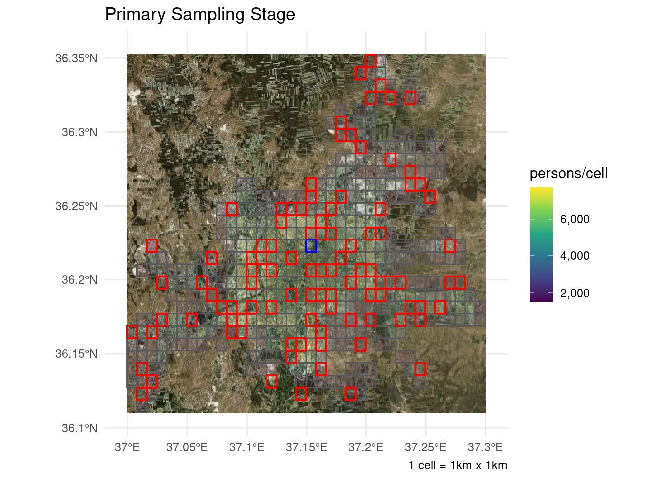

And here are the other two sampling stages (zooming in on the blue cell from above):

## Extract bounding box to get bing imagery
bbox <- ex %>%  st_bbox()

## Extract imagery background
map <- openmap(c(bbox$ymax,bbox$xmin), c(bbox$ymin,bbox$xmax), 
               zoom = 16,
               type =  "bing" ,
               mergeTiles = TRUE)



## OSM CRS :: "+proj=merc +a=6378137 +b=6378137 +lat_ts=0.0 +lon_0=0.0 +x_0=0.0 +y_0=0 +k=1.0 +units=m +nadgrids=@null +no_defs"
map.latlon <- openproj(map, projection = "+proj=longlat +ellps=WGS84 +datum=WGS84 +no_defs")


ssubg <- 
  
## option for google map background---   
#   get_googlemap(
#     center = ex %>% st_union() %>% st_centroid() %>% st_coordinates(),
#     zoom = 16,
#     scale = 1,
#     maptype = "satellite")
# 
# ssubg %>% 
#   ggmap() +

## Option for bing background  
  
  autoplot.OpenStreetMap(map.latlon)  +
  
  geom_sf(aes(fill = ppp), inherit.aes = FALSE, alpha = .15, 
          data = ppp100m %>% st_crop(ex) %>% st_as_sf()) +
  geom_sf(aes(geometry = ssugeometry), inherit.aes = FALSE,
          fill = NA, color = "red", alpha = .15, 
          data = s %>% st_filter(ex, .predicate = st_within)) +
  geom_sf(aes(geometry = tsugeometry), inherit.aes = FALSE,
          color = "blue", size = 2,
          data = s %>% st_filter(ex, .predicate = st_within)) +
  scale_fill_viridis_c(labels = scales::comma) +
  scale_x_continuous(labels = function(x) { str_c(x, "°", if_else(x >= 0, "E", "W")) }) +
  scale_y_continuous(labels = function(y) { str_c(y, "°", if_else(y >= 0, "N", "S")) }) +
  theme_minimal() +
  labs(title = "Secondary & Tertiary Sampling Stages",
       fill = "persons/cell", caption = "1 cell = 100m x 100m",
       x = NULL, y = NULL)

ssubg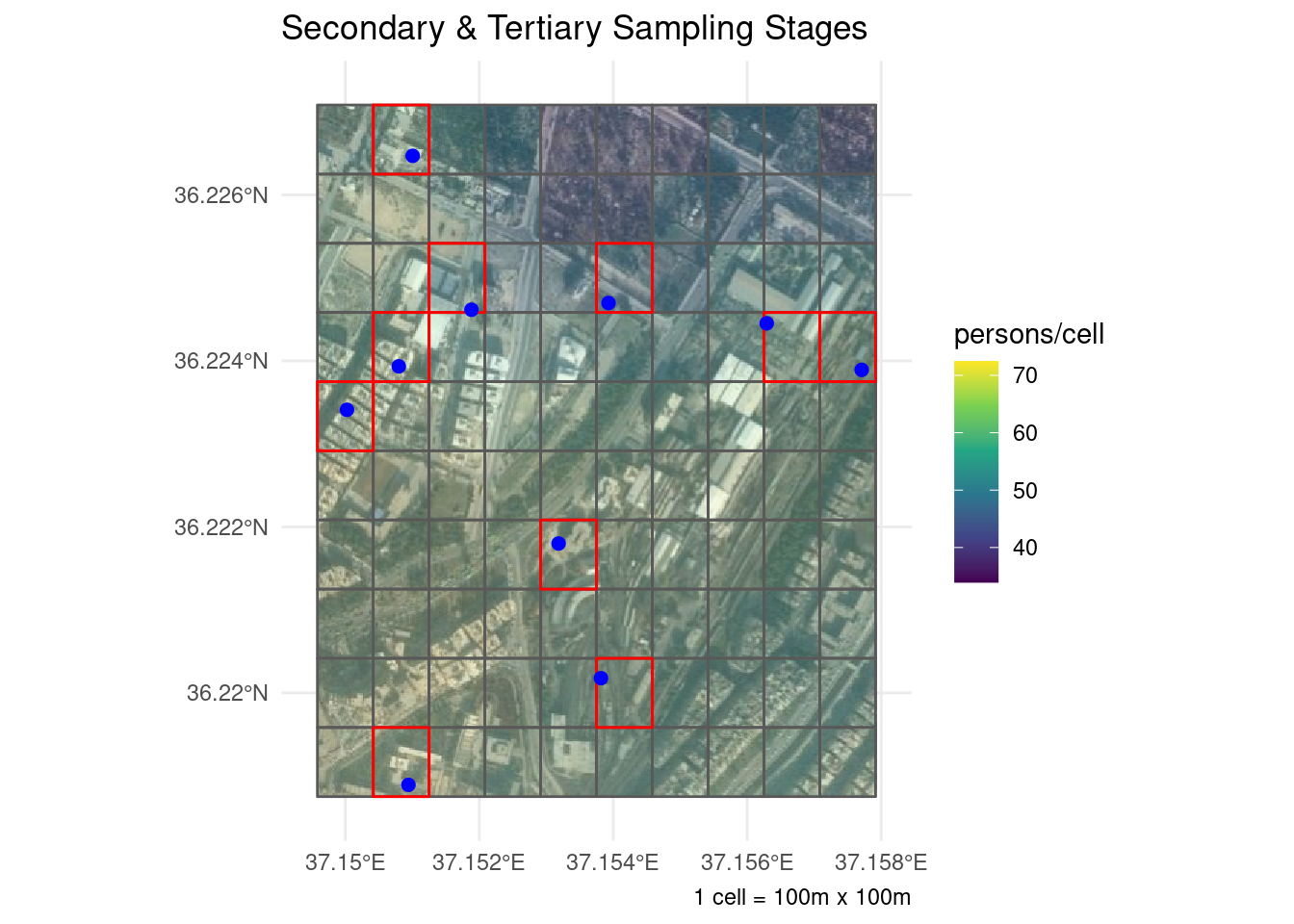

The blue dots above represent the random locations chosen in the third sampling stage. The rational behind this extra step is to avoid introducing bias into the sample by leaving the selection of dwelling units to the discretion of the enumerators.

One important implementation detail to note is the possibility that some of the sampled cells will have no dwellings in them. Machine learning methods aren’t perfect, and while errors cancel out in coarser grids, problems doesn’t cease to manifest at the more detailed levels. The way to deal with this is pretty much what we would do in any survey: enlarge our sample to account for likely non-response. It’s also possible to eyeball the sampled units against satellite imagery (as we have done here) to eliminate and replace empty cells before sending enumerators to the field.

Once the sample selection process is complete, the GPS coordinates of the sampled dwellings can be loaded onto the enumerators’ mobile data collection devices so they can easily find their way in the field.

Calculating Weights

Last but not least, we need to calculate our sample’s design weights before we wrap up.

The first and second stage inclusion probabilities are fairly straightforward:

s <- s %>% mutate(psup = psupop/aleppo$pop, ssup = ssupop/psupop)
s %>% 
  select( ssupop,ssuid, psup,ssup) %>% 
  rmarkdown::paged_table()

What about the third-stage selection of dwellings? One might assume that the selection is equiprobable since we’re simply drawing a random location within each cell but that is, in fact, incorrect.

To understand why, let’s run a simulation where we draw 10,000 random points from each of a few grid cells and see where they lead us to. We’ll zoom in to a small block in downtown Aleppo for the next illustration.

exloc <- st_point(c(37.118120, 36.214080))

ss <- 
  cbind(
    ppp1km_sf %>% 
      st_filter(exloc) %>% rename(psupop = ppp, psugeometry = geometry),
    ppp100m %>% 
      st_crop(exloc) %>% st_as_sf() %>% rename(ssupop = ppp, ssugeometry = geometry),
    tibble(
      tsugeometry = list(exloc)) %>% 
      st_sf(crs = st_crs(ppp1km_sf), sf_column_name = "tsugeometry")) %>% 
  st_set_geometry("ssugeometry") %>% 
  mutate(psup = psupop/aleppo$pop, ssup = ssupop/psupop)

exssu <- 
  ppp100m %>% 
  st_crop(ppp1km_sf %>% st_filter(ss)) %>% 
  st_as_sf() %>% 
  st_filter(ss) %>% 
  mutate(ssuid = row_number()) %>% 
  rename(ssupop = ppp, ssugeometry = geometry)

buildings <- 
  opq(st_bbox(exssu)) %>% 
  add_osm_feature("building") %>% 
  osmdata_sf() %>% 
  pluck("osm_polygons") %>% 
  transmute(tsuid = row_number()) %>% 
  rename(tsugeometry = geometry)

voronoi <- 
  exssu %>% 
  rowwise() %>% 
  mutate(dots = st_sample(ssugeometry, 10000) %>% st_as_sf() %>% list()) %>% 
  mutate(tsuid = 
           st_nearest_feature(
             st_set_crs(dots, st_crs(exssu)),
             buildings %>% st_crop(ssugeometry)) %>% 
           enframe(NULL, "id") %>% 
           left_join(buildings %>% st_crop(ssugeometry) %>% mutate(id = row_number())) %>% 
           pluck("tsuid") %>% 
           list()) %>% 
  unnest(c(dots, tsuid)) %>% 
  group_by(ssuid, tsuid) %>% 
  summarize(catchment = st_convex_hull(st_union(x))) %>% 
  ungroup() %>% 
  mutate_at(vars(catchment), st_sfc, crs = st_crs(exssu)) %>%
  st_as_sf()

voronoi <- voronoi %>% mutate(tsup = as.numeric(st_area(.)/st_area(exssu %>% head(1))))

voronoi %>% 
  ggplot() + 
  geom_sf(aes(fill = tsup)) +
  geom_sf(fill = "brown", data = buildings) +
  geom_sf(fill = NA, color = "blue", data = exssu) +
  expand_limits(fill = c(0, 1)) +
  scale_fill_viridis_c(labels = scales::percent) +
  scale_x_continuous(labels = function(x) { str_c(x, "°", if_else(x >= 0, "E", "W")) }) +
  scale_y_continuous(labels = function(y) { str_c(y, "°", if_else(y >= 0, "N", "S")) }) +
  theme_minimal() +
  labs(
    title = "Third-stage Inclusion Probabilities", 
    fill = "probability", caption = "1 cell = 100m x 100m")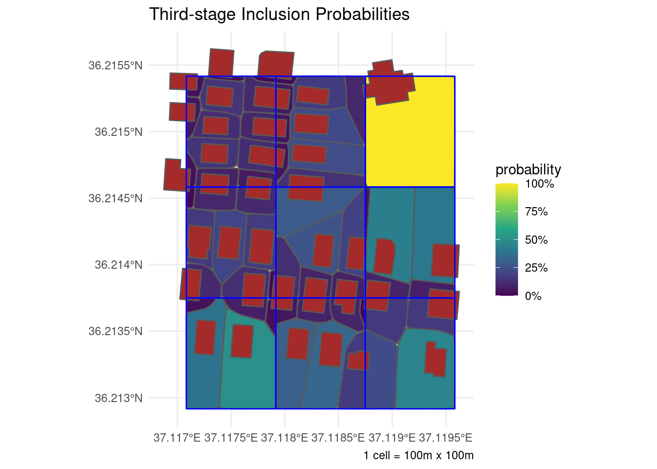

The technical term for this beautiful piece of abstract art is a Voronoi tessellation over the dwellings in each secondary sampling unit. What it’s telling us, basically, is that larger buildings and those in less crowded areas have more points leading to them than do the other buildings. As such, the third-stage inclusion probabilities should reflect the varying size of the catchment area between the different dwellings in a single grid cell.

Unfortunately, the process of producing these tessellations can only be partially automated. It requires someone to trace the outline of every dwelling intersecting the selected secondary sampling units (whether using shiny/leaflet or their favorite choice of GIS application) to feed the algorithm. This stage is essentially equivalent to the household listing step in any field survey except in this case it can be done completely from the office using freely available satellite imagery even before sending anyone to the field. We cheated here by purposefully selecting a block for which building outlines could be retrieved from OpenStreetMap. But that’s the exception rather than the norm. Most of the time building information simply isn’t available and has to be produced manually.

We can now update our sample to replace the random dot with its nearest building and include the third-stage sampling probability as well.

ss <- 
  ss %>% 
  st_set_geometry("tsugeometry") %>% 
  st_join(voronoi %>% select(tsuid, tsup)) %>% 
  mutate(tsugeometry = buildings %>% st_filter(voronoi %>% st_filter(tsugeometry)) %>% st_geometry())

Allowing us to produce normalized sample weights using the familiar formula:

ss <- 
  ss %>% 
  mutate(
    p = psup*ssup*tsup,
    wt = 1/p, wt = wt*length(wt)/sum(wt))

ss %>% 
  select(psupop, ssupop, psup,ssup,tsuid, tsup, p, wt  )%>% 
  rmarkdown::paged_table()

Needless to say, both ss and exssu in the above calculations should be replaced with s (the sample) in real-world implementation. The substitution was only done here to skirt around the problem of missing building data.

The final implementation detail to be aware of concerns fourth-stage selection procedures. While household survey protocols normally include guidance on selecting respondent units from multi-tenant dwellings, the issue warrants special attention in the context of geospatial sampling. The reason is that whereas in common sampling processes enumeration units are segmented so that dwellings would fall into one enumeration area or the other, in geospatial sampling from gridded population data it is not uncommon for dwellings to straddle the area between two or more grid cells. This complicates the calculation of selection probabilities as the same dwelling may enter the sample through more than one secondary sampling unit and selection probabilities need to be adjusted for that based on the probability calculation for sampling with replacement. One alternative would be to conceptually subdivide such dwellings so that, for example, if a building stretches across two cells, then even numbered apartments would be assigned to the Northern/Eastern cell and odd ones to the Southern/Western one. Standard procedures would then apply to select respondent units from among eligible apartments without affecting the calculation of weights.

Epilogue

The objective of this tutorial was to demonstrate the utility of marrying geospatial methods with household survey sampling techniques to produce representative samples in data poor environments. All too often, humanitarians have used the principle of “good enough” to justify fallback on methodically unsound approaches to needs assessment like convenience sampling and endless extrapolation from questionably designated key informants. Hopefully this tutorial has made the case that the challenges of data deprivation can be circumvented without compromising on methodical rigor.

This tutorial was inspired by recent work by the World Bank in fragility, conflict, and violence settings. Special thanks goes to Edouard Legoupil for his encouragement to write this post.