What is Conjoint analysis?
Conjoint analysis originated in mathematical psychology by psychometricians and was developed since the mid-sixties also by researchers in marketing and business. Conjoint analysis (CA) is often used to evaluate how people make decisions between a set of different options when considering a number of criteria at the same time (conjoint features; “trade-offs”). Rather than rating the importance of each attribute separately, participants rate their preferences for profiles or products with different combinations of the attributes or criteria. CA then allows to “decompose” or reverse-engineer these ratings into estimates of how important each criteria or attribute is to a participant’s ranking decisions.
In humanitarian data analysis, this technique can be quite relevant to organize expert consultations in order to get the relative weights (or relative contribution) of each sub-indicator value when creating composite indicator such as vulnerability scorecard. Conjoint analysis can speed up expert consultations by offering an objective mean to compile expert opinions.
As per OECD 10 Steps guide, one important elements to consider is the need to explore and compare different weighting approaches before making a decision on the final formula (i.e. also called sensitivity and robustness analysis).
As usual, R offers all the tools for that. Conjoint analysis can be done with the Conjoint Package, developed by the Department of Econometrics and Computer Science from Wrocław University of Economics. More details are available in their article: Conjoint analysis method and its implementation in conjoint R package.
Below is re-usable tutorial with reproducible code that should help any data analyst to quickly use this weighting discovery method.
Steps of the procedure for this example include:
Choosing the attributes/sub-indicators that are used to determine vulnerability scoring;
Determine the different potential levels for each attribute (i.e vulnerability scale attached to each answer option from sub-indicators) that indicate scoring of less vulnerable to more vulnerable;
Use fractional factorial design to generate a number of household profiles, each possessing unique combinations of the attributes;
- Build the expert consultation form where each expert will rate each household profile from low vulnerability to high vulnerability;
Review results and assess agreement level;
If necessary, relaunch the survey and iterate back to the previous step as much as needed;
Apply the importance level for each critiria as the weights to be used with the geometric mean aggregation for all indicators.
using <- function(...) {
    libs <- unlist(list(...))
    req <- unlist(lapply(libs,require,character.only = TRUE))
    need <- libs[req == FALSE]
    if (length(need) > 0) {
        install.packages(need)
        lapply(need,require,character.only = TRUE)
    }
}
using('conjoint','readr','DoE.base','ggpubr', 'dplyr', 'tidyr', 'AlgDesign', 'ggplot2',  'rlist', 'forcats', 'R.utils', 'png', 'grid', 'ggpubr', 'scales', 'cowplot', 'markdown', 'fpc', 'broom','openxlsx', 'GGally')
options(scipen = 999) # turn-off scientific notation like 1e+48

unhcr_style <- function() {
  font <- "Lato"
  ggplot2::theme(

#This sets the font, size, type and colour of text for the chart's title
  plot.title = ggplot2::element_text(family = font, size = 15, face = "bold", color = "#222222"),
#This sets the font, size, type and colour of text for the chart's subtitle,  as well as setting a margin between the title and the subtitle
  plot.subtitle = ggplot2::element_text(family = font, size = 12, margin = ggplot2::margin(9,0,9,0)),
  plot.caption = ggplot2::element_blank(),
#This sets the position and alignment of the legend, removes a title and backround for it and sets the requirements for any text within the legend. The legend may often need some more manual tweaking when it comes to its exact position based on the plot coordinates.
  legend.position = "top",
  legend.text.align = 0,
  legend.background = ggplot2::element_blank(),
  legend.title = ggplot2::element_blank(),
  legend.key = ggplot2::element_blank(),
  legend.text = ggplot2::element_text(family = font, size = 13, color = "#222222"),
#This sets the text font, size and colour for the axis test, as well as setting the margins and removes lines and ticks. In some cases, axis lines and axis ticks are things we would want to have in the chart
  axis.title = ggplot2::element_blank(),
  axis.text = ggplot2::element_text(family = font, size = 13, color = "#222222"),
  axis.text.x = ggplot2::element_text(margin = ggplot2::margin(5, b = 10)),
  axis.ticks = ggplot2::element_blank(),
  axis.line = ggplot2::element_blank(),
#This removes all minor gridlines and adds major y gridlines. In many cases you will want to change this to remove y gridlines and add x gridlines.
  panel.grid.minor = ggplot2::element_blank(),
  panel.grid.major.y = ggplot2::element_line(color = "#cbcbcb"),
  panel.grid.major.x = ggplot2::element_blank(),
#This sets the panel background as blank, removing the standard grey ggplot background colour from the plot
  panel.background = ggplot2::element_blank(),
#This sets the panel background for facet-wrapped plots to white, removing the standard grey ggplot background colour and sets the title size of the facet-wrap title to font size 22
  strip.background = ggplot2::element_rect(fill = "white"),
  strip.text = ggplot2::element_text(size  = 13,  hjust = 0)
  )
}

#Left align text
left_align <- function(plot_name, pieces){
  grob <- ggplot2::ggplotGrob(plot_name)
  n <- length(pieces)
  grob$layout$l[grob$layout$name %in% pieces] <- 2
  return(grob)
}

## functions used for utilities calculation - changed from initial package for better viz
m2v <- function(y,w=TRUE)
{
  y <- as.matrix(y)
  if (w) {S <- nrow(y); n <- ncol(y)} else {S <- ncol(y); n <- nrow(y)}
  tmp <- vector("numeric",S*n)
  k <- 0
  for (i in 1:S)
  {
    for (j in 1:n)
    {
      k = k + 1
      if (w) tmp[k] <- y[i,j] else tmp[k] <- y[j,i]
    }
  }
  ytmp <- as.data.frame(tmp)
  return(ytmp)
}

matexpand <- function(m, n, S, x)
{
  N <- n*S
  X <- matrix(0, N, m)
  k <- 1
  for (s in 1:S)
  {
    for (i in 1:n)
    {
      for (j in 1:m) {X[k,j] <- x[i,j]}
      k <- k + 1
    }
  }
  colnames(X) <- names(x)
  return(X)
}

caUtilities2   <-  function(y,x,z)
{
    options(contrasts = c("contr.sum","contr.poly"))
    outdec  <-  options(OutDec = "."); on.exit(options(outdec))
    options(OutDec = ",")
    y  <-  m2v(y)
    m  <-  length(x)
    n  <-  nrow(x)
    S  <-  nrow(y)/n
    xnms  <-  names(x)
    ynms  <-  names(y)
    xtmp  <-  paste("factor(x$",xnms,sep = "",paste(")"))
    xfrm  <-  paste(xtmp,collapse = "+")
    yfrm  <-  paste("y$",ynms,sep = "","~")
    frml  <-  as.formula(paste(yfrm,xfrm))
    Lj  <-  vector("numeric",m)
    for (j in 1:m) {Lj[j]  <-  nlevels(factor(x[[xnms[j]]]))}
    x  <-  as.data.frame(matexpand(m,n,S,x))
    camodel  <-  lm(frml)
    return(camodel)
    # print(summary.lm(camodel))
    # u  <-  as.matrix(camodel$coeff)
    # intercept  <-  u[1]
    # ul  <-  utilities(u,Lj)
    # utlsplot(ul,Lj,z,m,xnms)
    # uli  <-  c(intercept,ul)
    # return(uli)
}
Define the combined alternatives to be compared
The Joint Intersectoral Analysis Framework (JIAF) is a theoretical generic measurement framework to be used for Humanitarian needs assessment. It specifies three distinct and complementary components of humanitarian severity and vulnerability indexes:
- Basic Needs & Living standards
- Coping Capacity
- Well Being & Community integration
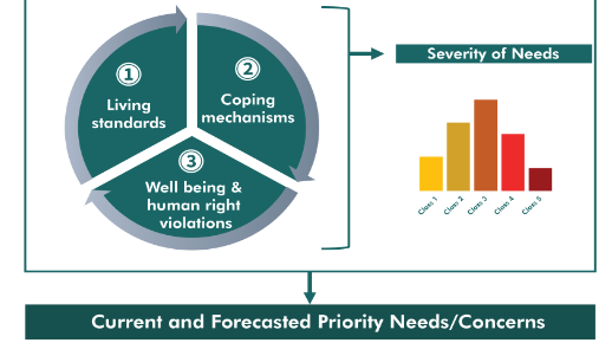
This generic model can be contextualized in each operations as different sub-indicators might be used for each of the 3 dimensions depending on cultural and political situations. Conjoint analysis will allow to discover the relative importance to be allocated for each sub-indicator.
# Declaration of features and feature values
basicneeds_indic <- c("Meals",
                      "Shelter",
                      "Water", #safely managed drinking water services inside accomodation
                      "Bathroom",
                      "Electricity") # electricity inside accomodation)

basicneeds_values.Meals <- c("One or less", "Two or more")
basicneeds_values.Shelter <- c("Owned or Rental", #"Owned or Rental (apartment or house) / Hotel",
                               "Hosted or Collective", #"Hosted Arrangement or Collective Accommodation in Transit/Reception center)",
                               "Spontaneous or Squatting") # "Spontaneous Arrangement or Street Squatting"
basicneeds_values.Water <- c("Safe Water", "No safe Water") # c("Safe Water in accomodation", "No safe Water in accomodation")
basicneeds_values.Bathroom <- c("Private",
                                "Collective or Shared toilets",
                                #"Collective or shared toilets and latrines",
                                "No bathroom")
basicneeds_values.Electricity <- c("Has electricity", "No electricity")

basicneeds_values <- c(basicneeds_values.Meals,
                       basicneeds_values.Shelter,
                       basicneeds_values.Water,
                       basicneeds_values.Bathroom,
                       basicneeds_values.Electricity)

# All concept generation
basicneeds <- expand.grid(
  Meals = basicneeds_values.Meals,
  Shelter = basicneeds_values.Shelter,
  Water = basicneeds_values.Water,
  Bathroom = basicneeds_values.Bathroom,
  Electricity = basicneeds_values.Electricity
)
coping_indic <- c("HH.Head",
"Dependency",
"Disability", # has household one member with disability
"Work", # at least one member in HH was able to get paid jobs in last month
"Neg.mechanism")
coping_values.HH.Head <- c("Male", "Elderly.Disabled", "Female", "Single", "Child")
coping_values.Dependency <- c("Low","Average", "High", "Full")
coping_values.Disability <- c("Has Disable", "No disable")
coping_values.Work <- c("One member Worked once in the week", "No work")
coping_values.Neg.mechanism <- c( "None",
"Stress", #"Working for in-kind instead of cash, Restrict food consumption, Borrow money, Sold assets, Increase Debt",
"Extreme") #"Sending children to other families or to work, Beging, Collecting food leftovers, Survival sex, Early mariage")
coping_values <- c(coping_values.HH.Head,
coping_values.Dependency,
coping_values.Disability,
coping_values.Work,
coping_values.Neg.mechanism)
# All concept generation
coping <- expand.grid(
HH.Head = coping_values.HH.Head,
Dependency = coping_values.Dependency,
Disability = coping_values.Disability,
Work = coping_values.Work,
Neg.mechanism = coping_values.Neg.mechanism
)wellbeing_indic <- c("Safety",
"Documentation",
"Communication",
"Isolation")
wellbeing_values.Safety <- c("Feel safe", "Not feeling safe")
wellbeing_values.Documentation <- c("Has essential documentation", "Missing document")
wellbeing_values.Communication <- c("Can access internet", "No access to internet")
wellbeing_values.Isolation <- c("Feel isolated", "Feel connected")
wellbeing_values <- c(wellbeing_values.Safety,
wellbeing_values.Documentation,
wellbeing_values.Communication,
wellbeing_values.Isolation)
# All concept generation
wellbeing <- expand.grid(
Safety = wellbeing_values.Safety,
Documentation = wellbeing_values.Documentation,
Communication = wellbeing_values.Communication,
Isolation = wellbeing_values.Isolation
)Select most relevant alternatives with Factorial Design
Instead of showing every possible combination of household profiles, fractional factorial design can be used to generate the fewest number of household profiles needed (each with a unique combination of the attribute levels).
In statistics, fractional factorial designs are experimental designs consisting of a carefully chosen subset (fraction) of the experimental runs of a full factorial design (i.e. all possible combinations of answers for a series of questions). The subset is chosen so as to exploit the sparsity-of-effects principle to expose information about the most important features of the problem studied, while using a fraction of the effort of a full factorial design in terms of experimental runs and resources. In other words, it makes use of the fact that many experiments in full factorial design are often redundant, giving little or no new information about the system.
In addition, the different profiles should be scanned to identify those specific interactions of criteria that are not rational (do not exist in the real world). Those should be removed manually.
# Selection of relevant concepts
selectedProfiles.basicneeds <- caFactorialDesign(data = basicneeds,
                                      type = 'fractional'
                                    )

## need to clean up some impossible profile
selectedProfiles.basicneeds <- selectedProfiles.basicneeds[ !(selectedProfiles.basicneeds$Shelter == "Spontaneous or Squatting" &
                              selectedProfiles.basicneeds$Bathroom == "Private")  , ]

selectedProfiles.basicneeds <- selectedProfiles.basicneeds[!(selectedProfiles.basicneeds$Shelter == "Hosted or Collective" &
                              selectedProfiles.basicneeds$Bathroom == "Private")  , ]

selectedProfiles.basicneeds <- selectedProfiles.basicneeds[!(selectedProfiles.basicneeds$Shelter == "Owned or Rental" &
                              selectedProfiles.basicneeds$Electricity == "No electricity")  , ]


# Checking if selected concepts are relevant for study
# corrselectedProfiles.basicneeds <- caEncodedDesign(selectedProfiles.basicneeds)
# print(cor(corrselectedProfiles.basicneeds))
# Selection of relevant concepts
selectedProfiles.coping <- caFactorialDesign(data = coping,
type ='fractional'
)
# Checking if selected concepts are relevant for study
# corrselectedProfiles.coping <- caEncodedDesign(selectedProfiles.coping)
# print(cor(corrselectedProfiles.coping))# Selection of relevant concepts
selectedProfiles.wellbeing <- caFactorialDesign(data = wellbeing,
type = 'fractional'
)
# Checking if selected concepts are relevant for study
# corrselectedProfiles.wellbeing <- caEncodedDesign(selectedProfiles.wellbeing)
# print(cor(corrselectedProfiles.wellbeing))## Build the expert consultation questionnaire in xlsform
Once we have the main profile options to compare, we can automatically generate the corresponding xlsform in order to build the expert consultation form.
Since we want the expert to rate each alternative, we will need a metric measurement, particularly a Likert scale. Likert scales are per default interval scales, which means that we would only have the knowledge of how much the overall utility would increase by changing the level of an attribute. We are also restricted to an interval scale due to the fact that we chose a part-worth model as well as fractional factorial design. A continuous or ratio variable would generally not be possible with a fractional factorial design or part worth model unless we can make some assumption about linearity and interactions which are simply unrealistic. But the advantage of a Likert scale is that it has proven to be more reliable in studies.
The rating of a run might look like this: - each expert is presented with a set of unique household profiles that represent different combinations of the attributes together (i.e. a “run from the experimental design”) - each expert then rates each profile with a number ranging from 1 to 9, where the higher number indicates that the household is highly vulnerable. 9 indicates extreme vulnerability, while 1 equals low vulnerability.
The questionnaire generation in xlsform can also be automatized with a script in order to save time. We predefined the survey introduction conjointSurvey.csv and the choices conjointShoices.csv
## survey intro and response can be predifined
survey <- read_csv("conjointSurvey.csv")
## Parsed with column specification:
## cols(
## type = col_character(),
## name = col_character(),
## label = col_character(),
## hint = col_character(),
## required = col_logical(),
## appearance = col_logical()
## )choices <- read_csv("conjointChoices.csv")## Parsed with column specification:
## cols(
## list_name = col_character(),
## name = col_character(),
## label = col_character()
## )## Aggregate profiles
profiles.basicneeds <- cbind("basicneeds", selectedProfiles.basicneeds)
profiles.basicneeds$type <- "select_one scale_basicneeds"
profiles.basicneeds$appearance <- "horizontal-compact"
profiles.basicneeds$hint <- " "
profiles.basicneeds$required <- "TRUE"
profiles.basicneeds$name <- paste0("basicneeds",row.names(profiles.basicneeds))
profiles.basicneeds$label <- paste0("Accomodation type is ",profiles.basicneeds$Shelter,",\n",
"there is ",profiles.basicneeds$Water,",\n",
"and ",profiles.basicneeds$Bathroom," can be accessed.\n",
"There is ",profiles.basicneeds$Electricity,"\n",
"and household members had ",profiles.basicneeds$Meals," meal(s) per day.")
profiles.coping <- cbind("coping", selectedProfiles.coping)
profiles.coping$type <- "select_one scale_coping"
profiles.coping$appearance <- "horizontal-compact"
profiles.coping$hint <- " "
profiles.coping$required <- "TRUE"
profiles.coping$name <- paste0("coping",row.names(profiles.coping))
profiles.coping$label <- paste0("Head of household is ",profiles.coping$HH.Head,",\n",
"household has ",profiles.coping$Dependency," dependency level.\n",
"and includes ",profiles.coping$Disability," can be accessed.\n",
"Members ",profiles.coping$Work,"\n",
"and have used ",profiles.coping$Neg.mechanism," negative coping mechanisms.")
profiles.wellbeing <- cbind("wellbeing", selectedProfiles.wellbeing)
profiles.wellbeing$type <- "select_one scale_wellbeing"
profiles.wellbeing$appearance <- "horizontal-compact"
profiles.wellbeing$hint <- " "
profiles.wellbeing$required <- "TRUE"
profiles.wellbeing$name <- paste0("wellbeing",row.names(profiles.wellbeing))
profiles.wellbeing$label <- paste0("Household members are ",profiles.wellbeing$Safety,".\n",
"They ",profiles.wellbeing$Isolation,".\n",
"They ",profiles.wellbeing$Documentation,".\n",
"They ",profiles.wellbeing$Communication,"\n")
profiles <- rbind(profiles.basicneeds[ ,c("type","name","label","hint","required","appearance")],
profiles.coping[ ,c("type","name","label","hint","required","appearance")],
profiles.wellbeing[ ,c("type","name","label","hint","required","appearance")])
rm(profiles.basicneeds,
profiles.coping,
profiles.wellbeing)
survey <- rbind(survey, profiles)
## Add a line to close the group
survey[ nrow(survey) + 1 , c("type")] <- "end_group"
## Creating setting for the xlsform
settings <- data.frame(c("Vulnerability Profiles Rating"))
names(settings)[1] <- "form_title"
settings$id_string <- "vulnerability_rating"
settings$style <- "theme-grid"
## Dave the form
xlsform <- openxlsx::createWorkbook()
openxlsx::addWorksheet(xlsform, "survey"); writeData(xlsform, "survey", survey)
openxlsx::addWorksheet(xlsform, "choices"); writeData(xlsform, "choices", choices)
openxlsx::addWorksheet(xlsform, "settings"); writeData(xlsform, "settings", settings)
openxlsx::saveWorkbook(xlsform, "conjoint_form.xlsx", overwrite = TRUE)For the time being, we can create a dummy dataset representing the consultation of 50 experts. We then merge the results with the design, so that each row represents an household with its features followed by the ratings it received by the experts.
set.seed(1234)
nexpert <- 50 # number of expert
Data <- data.frame(Expert = 1:nexpert)
Data$Expert <- as.factor(Data$Expert)
For Basic needs profile
## BasicNeeds
Data.basicneeds <- Data

for (run in 1:nrow(selectedProfiles.basicneeds)) {
  Data.basicneeds[,paste("Run",as.character(run), sep = "")] <- sample(c(1:9), nexpert, replace = TRUE)
}

# Merging FracDesign and Data.basicneeds
Data.basicneeds$Expert <- NULL
Data.basicneeds2 <- t(Data.basicneeds)
rownames(Data.basicneeds2) <- c(1:nrow(selectedProfiles.basicneeds))
Conjoint.basicneeds <- cbind(selectedProfiles.basicneeds, Data.basicneeds2)
For coping capacity profiles
## BasicNeeds
Data.coping <- Data

for (run in 1:nrow(selectedProfiles.coping)) {
  Data.coping[,paste("Run",as.character(run), sep = "")] <- sample(c(1:9), nexpert, replace = TRUE)
}

# Merging FracDesign and Data.coping
Data.coping$Expert <- NULL
Data.coping2 <- t(Data.coping)
rownames(Data.coping2) <- c(1:nrow(selectedProfiles.coping))
Conjoint.coping <- cbind(selectedProfiles.coping, Data.coping2)
For well being profiles
## wellbeing
Data.wellbeing <- Data

for (run in 1:nrow(selectedProfiles.wellbeing)) {
  Data.wellbeing[,paste("Run",as.character(run), sep = "")] <- sample(c(1:9), nexpert, replace = TRUE)
}

# Merging FracDesign and Data.wellbeing
Data.wellbeing$Expert <- NULL
Data.wellbeing2 <- t(Data.wellbeing)
rownames(Data.wellbeing2) <- c(1:nrow(selectedProfiles.wellbeing))
Conjoint.wellbeing <- cbind(selectedProfiles.wellbeing, Data.wellbeing2)
Utility values: estimating the Part-Worth Models
CA produces importance values and part-worth utility estimates. Importance values indicate the overall contribution of each attribute to how the profiles were rated (e.g. whether number of meals is more important in vulnerability scoring than access to safe water). Part-worth utility estimates the relative importance of each level within each attribute (e.g. the relative scoring of one or less meals vs. two or more meals a day). A higher utility estimate indicates that this level contributes to a higher vulnerability than the level with the lower utility estimate.
The part-worth model follows the idea of marginal utility from economics. It means it does not give an absolute value for the utility of an option, but rather assumes a reference alternative. The part-worth values for each expert can be calculated through multiple linear regression. The objective is estimate the preference share - i.e. how much a specific vulnerability criteria can contribute to the entire vulnerability score for a specific case.
A model is generated for each expert. The estimates of the linear regression are our part-worth utilities. Part-worth utilities are interval scale variables: for each categorical variable, one level is used as reference level. This means that for one level in each categorical variable no estimate will be shown because its value will be automatically 0.
The following code creates a data frame where each row represents a level of a variable and where each column represents an Expert.
#  get the numeric values for each part utility for each respondent.
PartUtilities <- as.data.frame(t(caPartUtilities(y = Data.basicneeds2,
                                 x = selectedProfiles.basicneeds,
                                 z = basicneeds_values)))

# Create dataframe with part-worthvalues
vars <- c("Intercept",
          rep("Meals",2),
          rep("Shelter",3),
          rep("Water",2),
          rep("Bathroom", 3),
          rep("Electricity",2))
lvls <- c("Intercept",
          as.character(levels(Conjoint.basicneeds$Meals)),
          as.character(levels(Conjoint.basicneeds$Shelter)),
          as.character(levels(Conjoint.basicneeds$Water)),
          as.character(levels(Conjoint.basicneeds$Bathroom)),
          as.character(levels(Conjoint.basicneeds$Electricity)))

Results <- data.frame(Variable = vars,Levels = lvls)
Results <- cbind(Results,PartUtilities )
Results[,"Average"] <- round(rowMeans(Results[,-c(1,2)]),digits = 1)
We can now visualize the results with ggplot2
myplots <- list()
count = 1

for (var in basicneeds_indic) {

  #var <- "Shelter"
  subs <- droplevels(subset(Results,Variable == var))
  subs$Levels <- reorder(subs$Levels,subs$Average)
  if (min(subs$Average) < 0) {
    subs$Average <- subs$Average + abs(min(subs$Average))
  }
  myplots[[count]]  <- ggplot(data = subs,aes(x = Levels, y = Average, group = 1)) +
    geom_line() +
    geom_point() +
    unhcr_style() + ## Insert UNHCR Style
    ## and the chart labels
    labs(title = paste0("Utilities level for ", var)) +
    theme(axis.text.x = element_text(angle = 45, vjust = 1, hjust = 1))
  count = count + 1

}

cowplot::plot_grid(plotlist = myplots, nrow = 3, ncol = 2)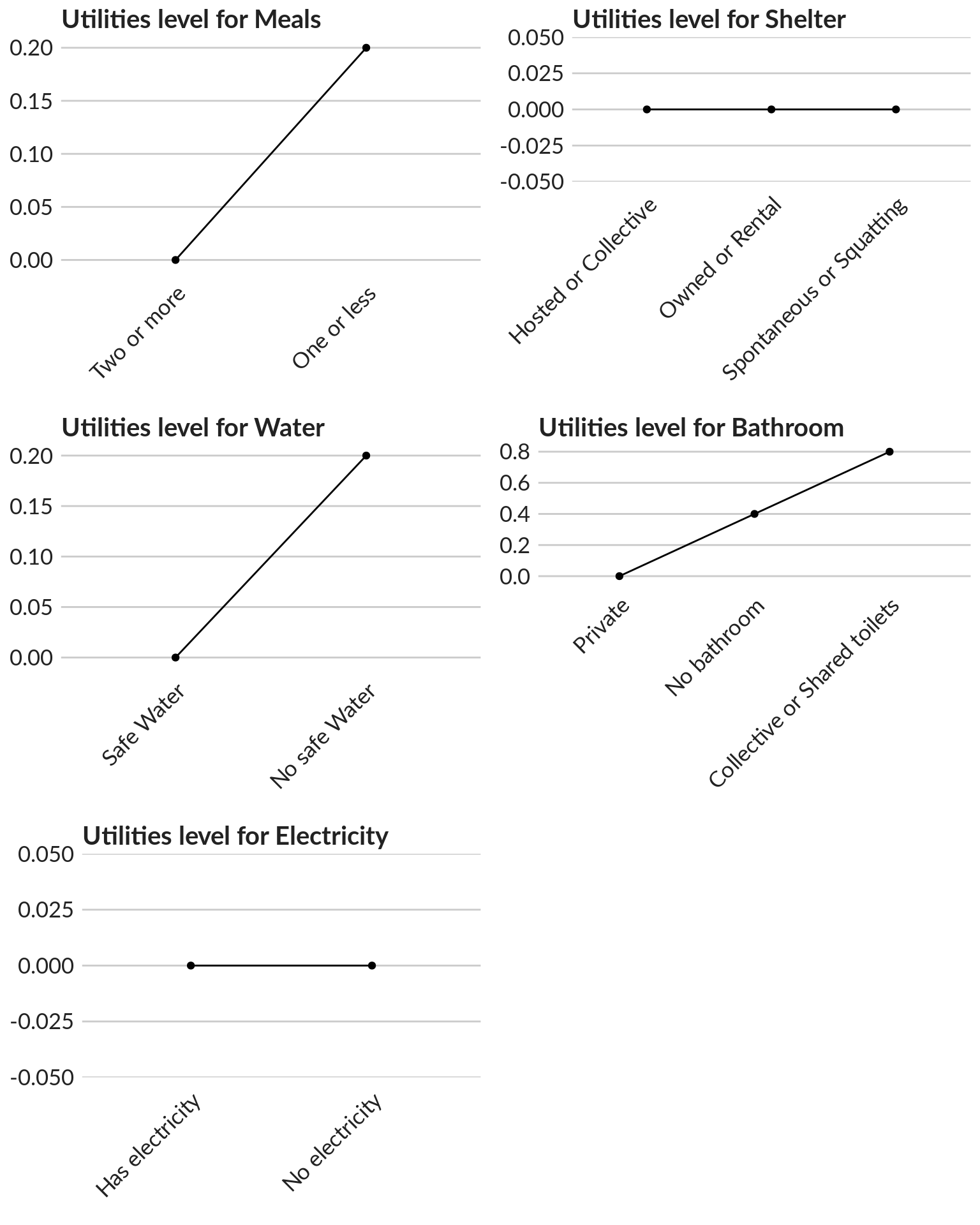
The standard deviation for each level allows to better understand how homogeneous the target group is with respect to one level. It might give us a hint on whether the preferences here considered are correct.
# The higher the utility value, the more importance that the expert places on that attribute’s level.


model  <-  caUtilities2(y = Data.basicneeds2 ,
                     x = selectedProfiles.basicneeds,
                     z = basicneeds_values)

model.tidy  <-  broom::tidy(model,
                          conf.int = TRUE,
                          conf.level = 0.95,
                          exponentiate = TRUE
)

model.tidy  <-  model.tidy[ !(is.na(model.tidy$term)), ]

Results$seq <- 1
for (i in 2:nrow(Results)) {
  if (Results[ i - 1 , c("Variable")] == Results[ i , c("Variable")])
  {Results[ i , c("seq")] <- Results[ i - 1 , c("seq")] + 1 } else {Results[ i , c("seq")] <- Results[ i , c("seq")]}

}

Results$term <- paste0("factor(x$", Results$Variable, ")", Results$seq )
Results$Levels2 <- paste0( Results$Variable, ": ", Results$Levels )
model.tidy2 <- merge(x = model.tidy, y = Results[ ,c("term", "Levels2")], by = "term", all.x = TRUE  )

### Chart showing the model
#ggcoef(model.,
plot1  <-  GGally::ggcoef(model.tidy2,
                  exponentiate = TRUE,
                color = "purple", shape = 18,  size = 3.5, exclude_intercept = TRUE,
                vline_color = "red", vline_linetype =  "solid",
                errorbar_color = "black", errorbar_height = .25,
                conf.level = 0.95, conf.int = TRUE,
                mapping = aes(x = estimate, y = Levels2)) +
  xlab("Influence factor for each variable") +
  ylab("") +
  labs(title = "Basic needs",
       subtitle =  "Contribution of answers to vulnerability scale",
       caption = "The black lines (also called 'whiskers') around the point represent the confidence interval \n for each variable to be included in the model (the shorter the line, the more experts are in agreement)",
       x = NULL, y = NULL) +
  unhcr_style() +
  theme( plot.caption = element_text(size = 8, hjust = 1),
         panel.grid.major.x = element_line(color = "#cbcbcb"),
         panel.grid.major.y = element_blank(),
         strip.text.x = element_text(size = 13))

ggpubr::ggarrange(left_align(plot1, c("subtitle", "title", "caption")), ncol = 1, nrow = 1)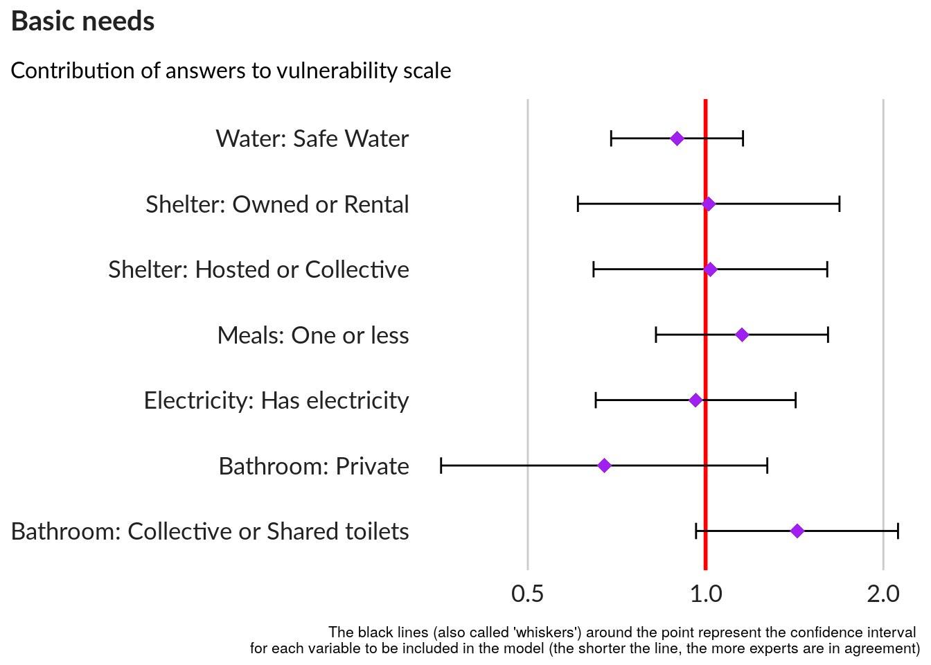
Importance of each criteria
We can now get the importance of each criteria. These importance values will then be used as the weights for each attribute inside each of our three dimensions. The importance values sum to 100%. In the example of the bar chart below, bathroom and shelter are more important than meals, water and electricity in rating vulnerability based on basic needs.
Importances.basicneeds <- as.data.frame(basicneeds_indic)
names(Importances.basicneeds)[1] <- "Variable"

Importances.basicneeds$Average <- caImportance(Data.basicneeds2,
                                    selectedProfiles.basicneeds)

plot1 <- ggplot(Importances.basicneeds,
       aes(x = reorder(Variable, Average), y = Average)) +
  geom_bar(stat = "identity",
           position = "identity",
           fill = "#0072bc") + # here we configure that it will be bar chart
  geom_label(aes(label = Average), size = 9, fill = "#0072bc" ,  color = "white", hjust = 1) +
  coord_flip() +
  scale_y_continuous(labels = function(x)paste(x, "%")) +
  unhcr_style() + ## Insert UNHCR Style
  ## and the chart labels
  labs(title = "Criteria Average importance related to Basic Needs Vulnerability scoring",
       subtitle = paste0("Conjoint Analysis from ", nexpert, " experts"),
       caption = "Dummy data",
       y = "") +
  theme(panel.grid.major.x = element_line(color = "#cbcbcb"),
        panel.grid.major.y = element_blank()) ### changing grid line that should appear

ggpubr::ggarrange(left_align(plot1, c("subtitle", "title")), ncol = 1, nrow = 1)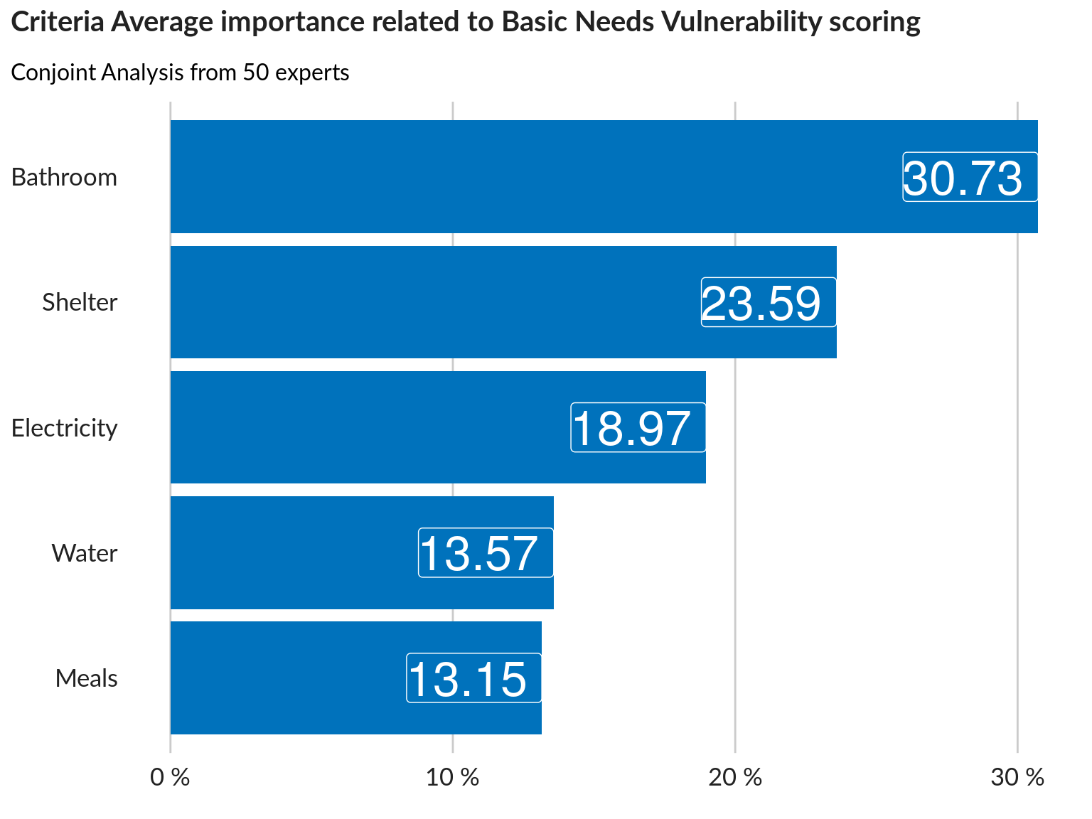
Segmentation of respondents
Segmentation using k-means method - division into 3 segments:
This will group experts according to their patterns of responses. This way we can identify if experts from different countries are giving different importance ratings compared to experts from other countries.
We can also see on the plot if there is a higher agreement between experts of a certain segment (segment 1, dots are closer together) vs. another.
segments <- caSegmentation(Data.basicneeds2,
                           selectedProfiles.basicneeds,
                           c = 3)

# print(segments$seg)
# plotcluster(segments$util,segments$sclu)

dcf <- discrcoord(segments$util,segments$sclu)
assignments <- augment(segments$segm,dcf$proj[,1:2])

plot1 <- ggplot(assignments) +
          geom_point(aes(x = X1,
                         y = X2,
                         color = .cluster)) +
        unhcr_style() + ## Insert UNHCR Style
        ## and the chart labels
        labs(title = "Profiling experts contribution",
             subtitle = paste0("K-Means Clustering of ", nexpert, " experts opinions"),
             caption = "Dummy data",
             color = "Cluster Assignment",
             y = "",
             x = "") +
        theme(panel.grid.major.x = element_line(color = "#cbcbcb"),
              panel.grid.major.y = element_line(color = "#cbcbcb"),
        axis.text.x  = ggplot2::element_blank(),
        axis.text.y  = ggplot2::element_blank())

ggpubr::ggarrange(left_align(plot1, c("subtitle", "title")), ncol = 1, nrow = 1)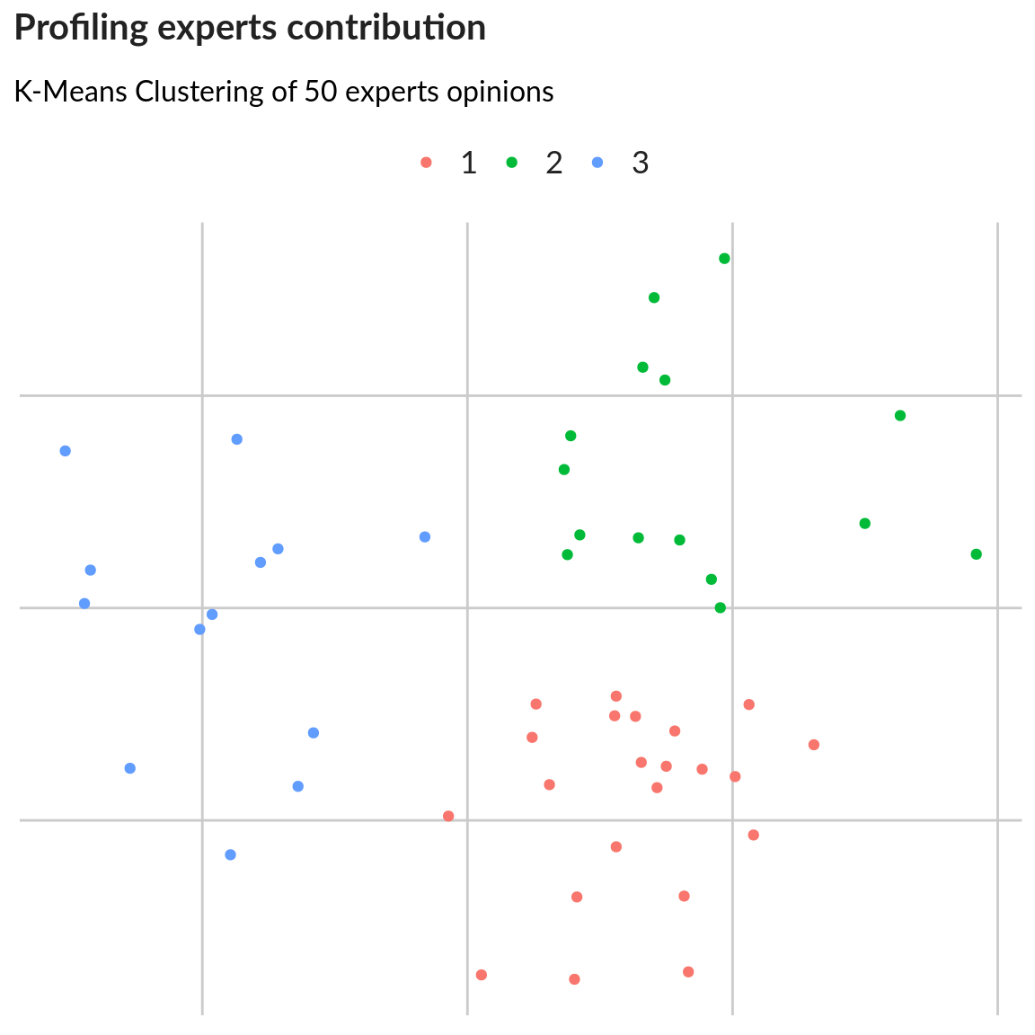
Share this post
Twitter
Google+
Facebook
Reddit
LinkedIn
StumbleUpon
Pinterest
Email