Simple Random Sampling

Simple random sampling is the cornerstone foundation of all sample designs. It’s implemented in dplyr using sample_n(). Here’s a draw of 1000 households:

universe %>% sample_n(size = 1000)

## # A tibble: 1,000 x 5
##    strata         ea    hh    safety    pcexp
##    <chr>          <chr> <chr> <chr>     <dbl>
##  1 Host community 128   12486 Safe     11196.
##  2 Host community 308   30522 Safe      5842.
##  3 Refugees       264   26485 Not safe  3529.
##  4 Host community 625   62127 Not safe  8179.
##  5 Host community 667   66311 Safe      9265.
##  6 Host community 259   25738 Safe     10715.
##  7 Host community 354   34970 Safe     11805.
##  8 Host community 172   16941 Safe      6745.
##  9 Host community 130   12736 Safe      9834.
## 10 Host community 476   47157 Safe     10941.
## # … with 990 more rows

Stratified Sampling

On to a slightly more sophisticated sample design. The beauty of dplyr is that it allows you to express in code the same exact steps you would follow when describing the method:

universe %>% 
  # partition the population into strata
  group_nest(strata) %>% 
  # for each stratum...
  rowwise() %>% 
  mutate(
    # calculate the required sample size
    samplesz = round(1000*nrow(data)/nrow(universe)),
    # then draw the sample
    sample = list(sample_n(data, size = samplesz))) %>% 
  select(-c(data, samplesz)) %>% 
  # et voila!
  unnest(sample)

## # A tibble: 1,000 x 5
##    strata         ea    hh    safety    pcexp
##    <chr>          <chr> <chr> <chr>     <dbl>
##  1 Host community 628   62409 Not safe 12276.
##  2 Host community 110   10667 Not safe  7144.
##  3 Host community 455   44932 Safe      9399.
##  4 Host community 125   12189 Not safe  7934.
##  5 Host community 584   57910 Safe      9732.
##  6 Host community 301   29859 Safe      9707.
##  7 Host community 455   44944 Safe      6846.
##  8 Host community 309   30631 Not safe  9303.
##  9 Host community 100   09825 Safe      8350.
## 10 Host community 289   28624 Safe      7961.
## # … with 990 more rows

That’s it for stratified sampling! For disproportionate stratification, just make sure to adjust samplesz accordingly.

Cluster Sampling

Clustering is fairly similar except this time we sample from the grouped table rather than within it.

universe %>% 
  # group the population by cluster
  group_nest(ea) %>% 
  # draw the desired number of clusters
  sample_n(size = 10) %>% 
  # and revert to a form that we can work with.
  unnest(data)

## # A tibble: 1,672 x 5
##    ea    strata         hh    safety    pcexp
##    <chr> <chr>          <chr> <chr>     <dbl>
##  1 634   Host community 62829 Not safe  9626.
##  2 634   Host community 62830 Not safe  8277.
##  3 634   Host community 62831 Not safe 12510.
##  4 634   Host community 62832 Not safe 11408.
##  5 634   Host community 62833 Not safe 11559.
##  6 634   Host community 62834 Not safe  9817.
##  7 634   Host community 62835 Safe     10844.
##  8 634   Host community 62836 Not safe 13357.
##  9 634   Host community 62837 Safe     10284.
## 10 634   Host community 62838 Not safe 13240.
## # … with 1,662 more rows

We could have also passed any measure of size to sample_n()’s weight argument for unequal probability sampling.

Multi-stage Sampling

Armed with the basics, we can compose the pieces to construct arbitrarily complex designs as we wish.

Here, for example, is the familiar two-stage design with probability proportional to size selection at first stage and equal sample allocation across strata:

mssample <- function(universe) {
  samplesz <- 1000
  strata_cnt <- length(unique(universe$strata))
  hh_per_cluster <- 10
  clusters_per_stratum <- samplesz/hh_per_cluster/strata_cnt
  
  msdata <- 
    universe %>% 
    group_nest(strata, ea) %>% 
    rowwise() %>% 
    mutate(psusz = nrow(data)) %>% 
    group_nest(strata) %>% 
    rowwise() %>% 
    mutate(stratasz = sum(data$psusz))

  stage1 <- 
    msdata %>% 
    rowwise() %>% 
    mutate(sample = list(tibble(slice_sample(data, n = clusters_per_stratum, weight_by = data[[1]]$psusz)))) %>% 
    select(-data) %>% 
    unnest(sample)
    
  stage2 <- 
    stage1 %>% 
    rowwise() %>% 
    mutate(sample = list(sample_n(data, size = hh_per_cluster))) %>% 
    select(-data) %>% 
    unnest(sample)
  
  s <- 
    stage2 %>% 
    mutate(
      p1 = psusz/stratasz, p2 = hh_per_cluster/psusz,
      p = p1 * p2,
      wt = 1/p, wt = wt/sum(wt) * length(wt)) %>% 
    select(-stratasz, -psusz, -p1, -p2, -p)
  
  s
}

(s <- mssample(universe))

## # A tibble: 1,000 x 6
##    strata         ea    hh    safety    pcexp    wt
##    <chr>          <chr> <chr> <chr>     <dbl> <dbl>
##  1 Host community 039   03884 Not safe 10981.  1.33
##  2 Host community 039   03852 Not safe  7743.  1.33
##  3 Host community 039   03909 Not safe  9167.  1.33
##  4 Host community 039   03886 Safe     10630.  1.33
##  5 Host community 039   03811 Safe     12105.  1.33
##  6 Host community 039   03802 Not safe  9659.  1.33
##  7 Host community 039   03923 Not safe  9134.  1.33
##  8 Host community 039   03794 Not safe 11369.  1.33
##  9 Host community 039   03835 Safe      8881.  1.33
## 10 Host community 039   03915 Safe     10969.  1.33
## # … with 990 more rows

We’ve stored this design and its output so we can reuse them in the second half of this tutorial. Also note that we’ve added normalized weights to our sample in the last step so that we could draw valid inferences from our sample.

Point Estimation

Point estimation refers to the calculation of sums, averages, ratios, etc… from sample data.

For estimates involving categorical variables, dplyr’s count() already supports a wt argument for weighted calculations.

s %>% count(strata, safety, wt = wt) %>% group_by(strata) %>% mutate(p = n/sum(n)*100)

## # A tibble: 4 x 4
## # Groups:   strata [2]
##   strata         safety       n     p
##   <chr>          <chr>    <dbl> <dbl>
## 1 Host community Not safe  186.  28. 
## 2 Host community Safe      478.  72  
## 3 Refugees       Not safe  216.  64.2
## 4 Refugees       Safe      121.  35.8

Which is basically what we had specified when constructing our synthetic data: 70% of the host community feel safe in their neighborhoods whereas only 40% of the refugee population share the sentiment.

Actually, since our sample is self-weighting within each strata, the results would have come back the same with or without weights. Let’s look at the overall totals to see why weights are needed:

left_join(
  s %>% count(safety, wt = wt, name = "n.weighted") %>% mutate(p.weighted = n.weighted/sum(n.weighted)*100),
  s %>% count(safety, name = "n.unweighted") %>% mutate(p.unweighted = n.unweighted/sum(n.unweighted)*100))

## # A tibble: 2 x 5
##   safety   n.weighted p.weighted n.unweighted p.unweighted
##   <chr>         <dbl>      <dbl>        <int>        <dbl>
## 1 Not safe       402.       40.2          461         46.1
## 2 Safe           598.       59.8          539         53.9

Now compare that to the census:

universe %>% count(safety) %>% mutate(p = n/sum(n)*100)

## # A tibble: 2 x 3
##   safety       n     p
##   <chr>    <int> <dbl>
## 1 Not safe 40673  40.7
## 2 Safe     59311  59.3

And you could see that our weighted estimates are more in line with what we should have gotten.

What about point estimates involved continuous variables? Unfortunately there’s no convenience function similar to count() for those. That means we’ll have to fall back on the usual group+summarize workflow:

s %>% group_by(strata) %>% summarize(pcexp = weighted.mean(pcexp, wt))

## # A tibble: 2 x 2
##   strata         pcexp
##   <chr>          <dbl>
## 1 Host community 9947.
## 2 Refugees       5025.

Ground-truth:

universe %>% group_by(strata) %>% summarize(pcexp = mean(pcexp))

## # A tibble: 2 x 2
##   strata         pcexp
##   <chr>          <dbl>
## 1 Host community 9977.
## 2 Refugees       4979.

Close enough, with slight deviations because of sampling error… which brings us to the last part of this tutorial.

Variance Estimation

When producing estimates from sample data, we’re normally interested in more than just the point estimates. We also want to know how accurate our estimates are. This is the domain of variance estimation.

Let’s start by producing the actual sampling distribution of our mean per-capita expenditure statistic. We can do that since we’re working with simulated data. It wouldn’t otherwise be possible in the real world.

samplingdist <- 
  map_dfr(
    1:500,
    function(x) {
      mssample(universe) %>% 
        { 
          bind_rows(
            group_by(., strata) %>% summarize(pcexp = weighted.mean(pcexp, wt)),
            group_by(., strata = "Everyone") %>% summarize(pcexp = weighted.mean(pcexp, wt)))
        }
    })

Which tells us that our point estimates and standard errors should be:

(est_universe <- samplingdist %>% group_by(strata) %>% summarize(est = mean(pcexp), se = sd(pcexp)))

## # A tibble: 3 x 3
##   strata           est    se
##   <chr>          <dbl> <dbl>
## 1 Everyone       8295.  66.1
## 2 Host community 9979.  93.5
## 3 Refugees       4976.  60.0

We had gotten to those point estimates in the previous section. Our job now is to try to reproduce the standard error se from nothing but the sample data.

Most software approaches variance estimation using analytical methods grounded in some smart mathematical approximations. We’ll take a more (brute-force) computational approach based on the bootstrap here. The bootstrap, for those not familiar with it, is the idea of resampling with replacement from sample data to approximate the sampling distribution of the target statistic. See section 2 of this article for more details on the how and why of bootstrapping.

We could implement the bootstrap ourselves using rerun() and sample_n() with replace = TRUE but instead we’re going to pull in tidymodels and use rsample::bootstraps(). It’s more convenient, idiomatic, and you’ll probably have tidymodels loaded in your workspace anyway if you’re planning on running any models on your survey data.

library(tidymodels)

b <- s %>% group_nest(strata, ea) %>% bootstraps(times = 500, strata = strata)

b <- 
  b %>% 
  rowwise() %>% 
  mutate(
    stats = 
      analysis(splits) %>% 
      unnest(data) %>% 
      { 
        bind_rows(
          group_by(., strata) %>% summarize(pcexp = weighted.mean(pcexp, wt)),
          group_by(., strata = "Everyone") %>% summarize(pcexp = weighted.mean(pcexp, wt)))
      } %>% 
      list()
  )

(est_sample <- 
  b %>% 
  select(stats) %>% 
  unnest(stats) %>% 
  group_by(strata) %>% 
  summarize(est = mean(pcexp), se = sd(pcexp)))

## # A tibble: 3 x 3
##   strata           est    se
##   <chr>          <dbl> <dbl>
## 1 Everyone       8290.  59.7
## 2 Host community 9947.  85.1
## 3 Refugees       5024.  56.9

The key thing to keep in mind is that the bootstrap sample should resemble the original sample in the way it is drawn. Meaning, if we had drawn clusters from within strata in the original sample, then we should resample clusters within strata for the bootstrap.

Let’s see how our estimates stack up against the actual values we had calculated earlier.

bind_rows("sampling distribution" = est_universe, "bootstrap" = est_sample, .id = "src") %>% 
  ggplot(aes(x = est, y = strata, xmin = est - 2*se, xmax = est + 2*se, color = src)) +
  geom_point(position = position_dodge(-.5), size = 3) +
  geom_errorbarh(position = position_dodge(-.5), height = .5) +
  theme_minimal() +
  labs(x = NULL, y = NULL, color = NULL,
       title = "Estimated per-capita expenditures",
       subtitle = "Mean & 95% confidence interval")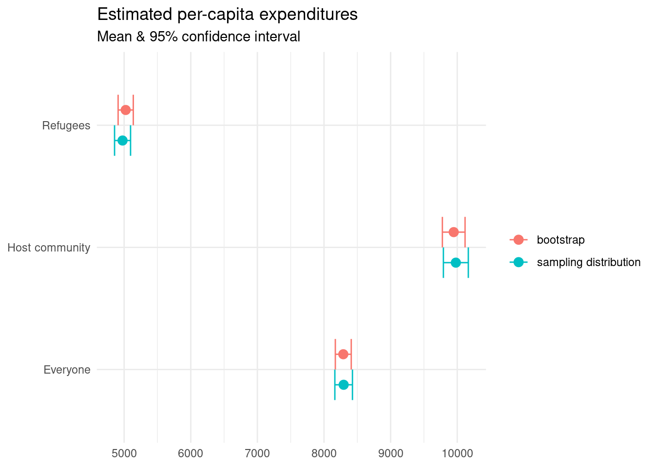

Confirming that our estimates line up with what they should be.