Bar Chart Race for Refugees

March 24, 2019 Edouard Legoupil

9 minutes read

“Bar Chart Race” are a specific type of bar chart that moves to show rankings over time. It became recently a quite popular approach to bring a storytelling elements within a longitudinal dataset. Readers are suggested to connect and combine what they see on the chart with other qualitive elements that they know about (elements of history). By using the allegory of F1 Race, it gives a very dynamic dimension.

You can check below a series of Viz on different issues:

10 most populous cities in the world from 1500-2018:

10 most populous cities in the world from 1500-2018. #dataviz https://t.co/vtGEBVLdYk pic.twitter.com/uvIkuE4VDI
— Randy Olson (@randal_olson) March 19, 2019

10 largest CO2 emitter

Bar Chart Race for CO2

The changing ranks of the 10 largest CO2 emitters in the world since 1850.

Fascinating to see nations rise, fall & rise again in their yearly emissions*

See how the UK dominates the C19th & US the 20th.

Then watch China surge ahead after 2005… pic.twitter.com/mFLuHB8kTw
— Simon Evans (@DrSimEvans) March 21, 2019

10 most expensive cities

Very impressed by the ‘bar chart race’ template from @f_l_o_u_r_i_s_h. It doesn't have @jburnmurdoch's awesome multipurpose map, but the legend toggle is a lovely touch (1/3) pic.twitter.com/RbjxTC7V5W
— Alex Selby-Boothroyd (@AlexSelbyB) March 22, 2019

With R, it’s fairly easy to reproduce such vis - We will show here how to use gganimate R packages to display evolution of refugees & IDP’s number over time based on UNHCR statistics

## Getting all necessary package

using <- function(...) {
    libs <- unlist(list(...))
    req <- unlist(lapply(libs,require,character.only = TRUE))
    need <- libs[req == FALSE]
    if (length(need) > 0) { 
        install.packages(need)
        lapply(need,require,character.only = TRUE)
    }
}


using("tidyverse","gganimate","gghighlight","ggpubr")

## loading libraries plus functions

library(tidyverse)
library(gganimate)
library(gghighlight)
library(ggpubr)


## a little help function to better format number
format_si <- function(...) {
  function(x) {
    limits <- c(1e-24, 1e-21, 1e-18, 1e-15, 1e-12,
                1e-9,  1e-6,  1e-3,  1e0,   1e3,
                1e6,   1e9,   1e12,  1e15,  1e18,
                1e21,  1e24)
    prefix <- c("y",   "z",   "a",   "f",   "p",
                "n",   "",   "m",   " ",   "k",
                "M",   "G",   "T",   "P",   "E",
                "Z",   "Y")

    # Vector with array indices according to position in intervals
    i <- findInterval(abs(x), limits)

    # Set prefix to " " for very small values < 1e-24
    i <- ifelse(i == 0, which(limits == 1e0), i)

    paste(format(round(x/limits[i], 1),
                 trim = TRUE, scientific = FALSE, ...),
          prefix[i])
  }
}

Let’s now download the data from UNHCR popstat API

# Time series
#url <- paste( 'http://popstats.unhcr.org/en/time_series.csv') 
#download.file(url, destfile = "unhcr_popstats_export_time_series_all_data.csv" )

Reshape the data to get the top 10 for each year using tidyverse

time_series <- read.csv("unhcr_popstats_export_time_series_all_data.csv", skip = 3) 
## rename the country and make sure Value is a number...
names(time_series)[2] <- "Country"

## make sure Value is numeric
time_series$Value <- as.integer(as.character(time_series$Value))

## Check what population type we have there and subset accordingly
#levels(time_series$Population.type)

time_series2 <- time_series[ time_series$Population.type %in% c("Refugees (incl. refugee-like situations)", "Internally displaced persons" ), ]

time_series2$Country <- as.character(time_series2$Country)
time_series2$Country[time_series2$Country == "C\xf4te d'Ivoire"] <- "Cote d'Ivoire" 
time_series2$Country <- as.factor(time_series2$Country)

time_series$Population.type <- as.factor(as.character(time_series$Population.type))

## Remove unknow countries or blanks
time_series2 <- time_series2[ !(time_series2$Country %in% c("Various/Unknown" )), ]

## Remove if value is 0 or NA
time_series2 <- time_series2[ !(is.na(time_series2$Value)), ]
time_series2 <- time_series2[ time_series2$Value != 0, ]

## Now get the rank from high to low for all countries per  year and population type
rank_data <- time_series2 %>%
  group_by(Year, Population.type, Country) %>%
  summarise(Value2 = sum(Value) ) 


#str(as.data.frame(rank_data))
rank_data <- as.data.frame(rank_data)

rank_data2 <- rank_data %>%
  group_by(Year, Population.type) %>%
  
  ## Tried first rank but did not provided ranks as integer... 
  # mutate(ordering = rank(-Value), ties.method = "min") %>%
  
  mutate(ordering = rank(-Value2)) %>%
  ungroup() 

## check our value for rank -- Note that there are different tie method
#levels(as.factor(rank_data$ordering))

## need to fix manually issue when ex-aequo rank rank = 8.5 

## In 1962
rank_data2$ordering[rank_data2$ordering == 10 &
                      rank_data2$Year == "1962" &
                      rank_data2$Population.type %in% c("Refugees (incl. refugee-like situations)")] <- 11

rank_data2$ordering[rank_data2$ordering == 8.5 &
                      rank_data2$Year == "1962" &
                      rank_data2$Country == "Burundi" &
                      rank_data2$Population.type %in% c("Refugees (incl. refugee-like situations)")] <- 9

rank_data2$ordering[rank_data2$ordering == 8.5 &
                      rank_data2$Year == "1962" &
                      rank_data2$Country == "Austria" &
                      rank_data2$Population.type %in% c("Refugees (incl. refugee-like situations)")] <- 10


## In 1978
rank_data2$ordering[rank_data2$ordering == 10 &
                      rank_data2$Year == "1978" &
                      rank_data2$Population.type %in% c("Refugees (incl. refugee-like situations)")] <- 11

rank_data2$ordering[rank_data2$ordering == 8.5 &
                      rank_data2$Year == "1978" &
                      rank_data2$Country == "Viet Nam" &
                      rank_data2$Population.type %in% c("Refugees (incl. refugee-like situations)")] <- 9

rank_data2$ordering[rank_data2$ordering == 8.5 &
                      rank_data2$Year == "1978" &
                      rank_data2$Country == "United Kingdom" & 
                      rank_data2$Population.type %in% c("Refugees (incl. refugee-like situations)")] <- 10


## and for IPDs

rank_data2$Country <- as.character(rank_data2$Country)

## In 1996
rank_data2$ordering[rank_data2$ordering == 10 &
                      rank_data2$Year == "1996" &
                      rank_data2$Population.type %in% c("Internally displaced persons")] <- 11

rank_data2$ordering[rank_data2$ordering == 9.5 &
                      rank_data2$Year == "1996" &
                      rank_data2$Country == "Somalia" &
                      rank_data2$Population.type %in% c("Internally displaced persons")] <- 11


rank_data2$Country[rank_data2$ordering == 9.5 &
                      rank_data2$Year == "1996" &
                      rank_data2$Country == "Sri Lanka" & 
                      rank_data2$Population.type %in% c("Internally displaced persons")] <- "Sri Lanka / Somalia"

rank_data2$ordering[rank_data2$ordering == 9.5 &
                      rank_data2$Year == "1996" &
                      rank_data2$Country == "Sri Lanka / Somalia" & 
                      rank_data2$Population.type %in% c("Internally displaced persons")] <- 10

## in 1997
rank_data2$ordering[rank_data2$ordering == 10 &
                      rank_data2$Year == "1997" &
                      rank_data2$Population.type %in% c("Internally displaced persons")] <- 11

rank_data2$ordering[rank_data2$ordering == 9.5 &
                      rank_data2$Year == "1997" &
                      rank_data2$Country == "Somalia" &
                      rank_data2$Population.type %in% c("Internally displaced persons")] <- 11


rank_data2$Country[rank_data2$ordering == 9.5 &
                      rank_data2$Year == "1997" &
                      rank_data2$Country == "Sri Lanka" & 
                      rank_data2$Population.type %in% c("Internally displaced persons")] <- "Sri Lanka / Somalia"

rank_data2$ordering[rank_data2$ordering == 9.5 &
                      rank_data2$Year == "1997" &
                      rank_data2$Country == "Sri Lanka / Somalia" & 
                      rank_data2$Population.type %in% c("Internally displaced persons")] <- 10


rank_data2$Country <- as.factor(rank_data2$Country)

# Filter only top 10 
rank_data2 <- rank_data2[rank_data2$ordering <= 10, ]
#rank_data$Year = as.Date(as.character(rank_data$Year), format = "%Y")


## Regnerate facors modality - 
rank_data2$Country <- as.factor(as.character(rank_data2$Country))
# levels(as.factor(rank_data2$Country))
## Double checking country name
#table(time_series2$Country, useNA = "ifany")

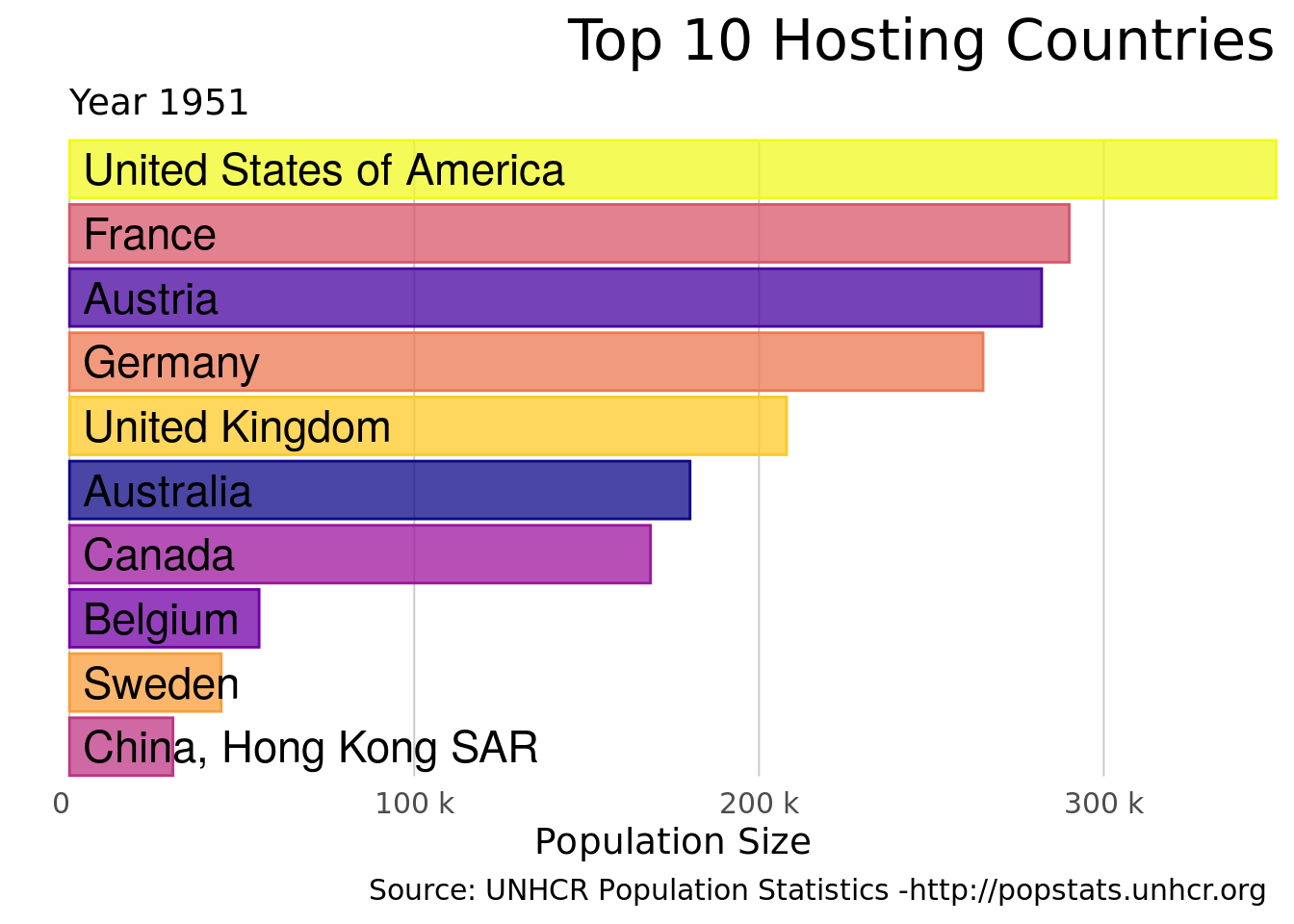
and now visualise

ggplot(rank_data2[ rank_data2$Year == 1951 & rank_data2$Population.type %in% c("Refugees (incl. refugee-like situations)"), ]) +
  geom_bar(aes(y = Value2,  x =   reorder(ordering, desc(ordering)),
               group = Country ,color = Country, fill = Country), alpha = 0.75, stat = "identity") +
  
  geom_label(aes(y = 0 , x =  reorder(ordering, desc(ordering)), label = Country),
             hjust = 0,
             vjust = 0.5,
             fill = NA,
             label.size = NA,
             family = "Helvetica",
             size = 6) +

  coord_flip(clip = "off", expand = FALSE) +
  scale_color_viridis_d(option = "plasma" ) +
  scale_fill_viridis_d(option = "plasma") +
  scale_y_continuous(labels = format_si()) +
  theme_minimal(14, "Avenir") +
  
  guides(color = F, fill = F) +
  labs(title =  "Top 10 Hosting Countries",
       subtitle = 'Year 1951',
       y = "Population Size",
       x = "",
       caption =  "Source: UNHCR Population Statistics -http://popstats.unhcr.org ") +
  theme(plot.title = element_text(hjust = 1, size = 22),
        axis.ticks.y = element_blank(),
        axis.text.y  = element_blank(), 
        panel.background  = element_blank(), 
        panel.grid = element_blank(),
        plot.background = element_blank(),
        legend.position = "bottom",
        panel.grid.major.x = element_line(color = "#cbcbcb"), 
        panel.grid.major.y = element_blank())

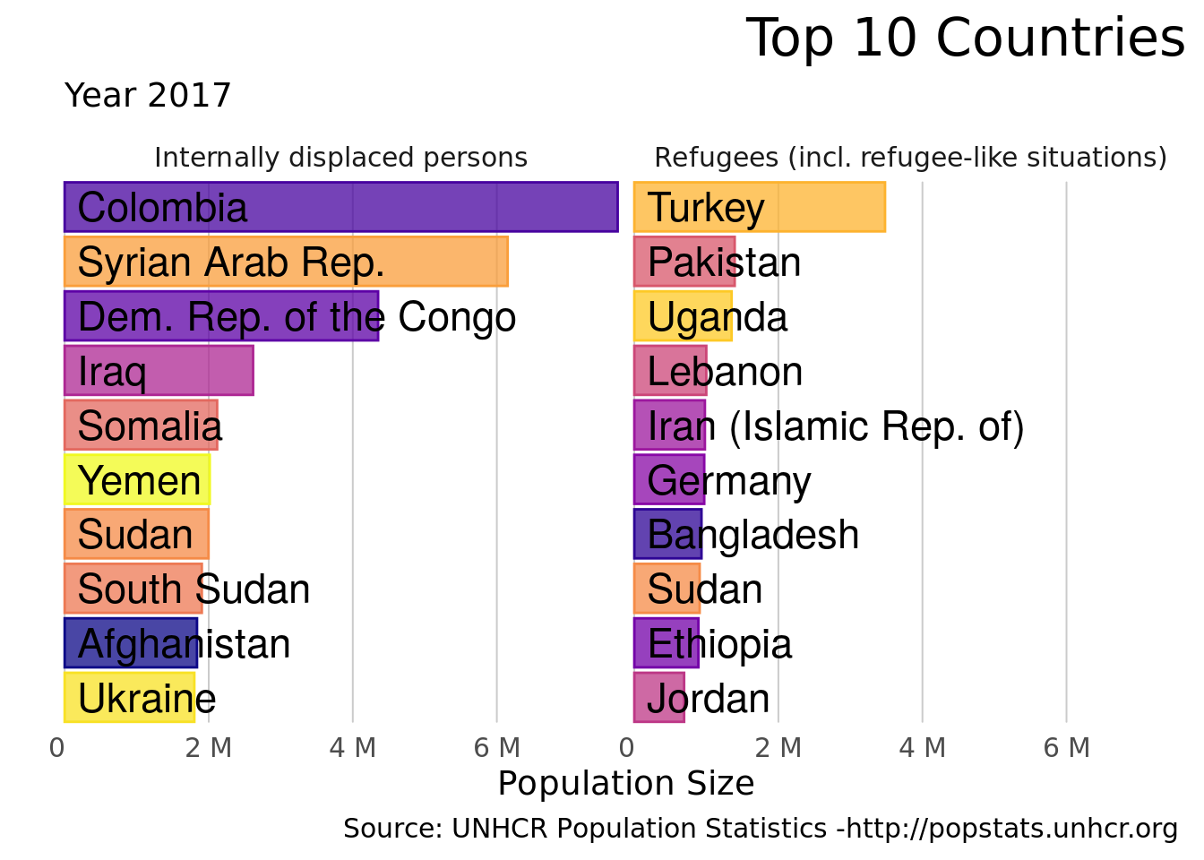
Faceting by Population Group for 2017

ggplot(rank_data2[ rank_data2$Year == 2017, ]) +
  geom_bar(aes(y = Value2,  x =   reorder(ordering, desc(ordering)),
               group = Country ,color = Country, fill = Country), alpha = 0.75, stat = "identity") +
  
  geom_label(aes(y = 0 , x =  reorder(ordering, desc(ordering)), label = Country),
             hjust = 0,
             vjust = 0.5,
             fill = NA,
             label.size = NA,
             family = "Helvetica",
             size = 6) +
  
  #facet_wrap( ~ Population.type) +
  facet_grid(. ~ Population.type) +
  coord_flip(clip = "off", expand = FALSE) +
  scale_color_viridis_d(option = "plasma" ) +
  scale_fill_viridis_d(option = "plasma") +
  scale_y_continuous(labels = format_si()) +
  theme_minimal(14, "Avenir") +
  
  guides(color = F, fill = F) +
  labs(title =  "Top 10 Countries",
       subtitle = 'Year 2017',
       y = "Population Size",
       x = "",
       caption =  "Source: UNHCR Population Statistics -http://popstats.unhcr.org ") +
  theme(plot.title = element_text(hjust = 1, size = 22),
        axis.ticks.y = element_blank(),
        axis.text.y  = element_blank(), 
        panel.background  = element_blank(), 
        panel.grid = element_blank(),
        plot.background = element_blank(),
        legend.position = "bottom",
        panel.grid.major.x = element_line(color = "#cbcbcb"), 
        panel.grid.major.y = element_blank())

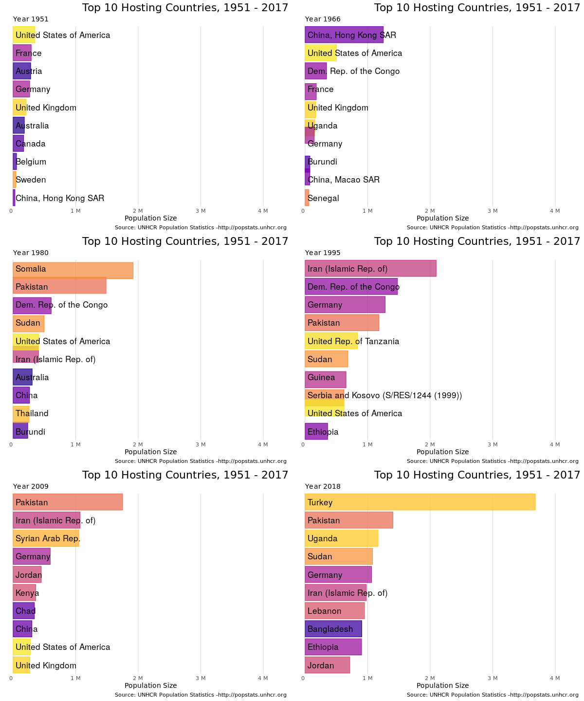
and animate…. the bar chart race…

p <- ggplot(rank_data2[rank_data2$Population.type %in% c("Refugees (incl. refugee-like situations)"), ]) +
  geom_bar(aes(y = Value2,  x =   reorder(ordering, desc(ordering)),
               group = Country ,color = Country, fill = Country), alpha = 0.75, stat = "identity") +
  
  geom_label(aes(y = 0 , x =  reorder(ordering, desc(ordering)), label = Country),
             hjust = 0,
             vjust = 0.5,
             fill = NA,
             label.size = NA,
             family = "Helvetica",
             size = 6) +
  
  coord_flip(clip = "off", expand = FALSE) +
  scale_color_viridis_d(option = "plasma" ) +
  scale_fill_viridis_d(option = "plasma") +
  scale_y_continuous(labels = format_si()) +
  theme_minimal(14, "Avenir") +
  #facet_wrap( ~ Population.type) +
  #facet_grid(. ~ Population.type) +
  
  ## get the animation per year... #, nframes = 250, fps = 10, end_pause = 20
  transition_time(Year ) +
  ease_aes('cubic-in-out') + 
 # enter_fade() +
 # exit_fade() +
  #view_follow(fixed_y = TRUE) +
  
  guides(color = F, fill = F) +
  labs(title =  "Top 10 Hosting Countries, 1951 - 2017",
       subtitle = 'Year {frame_time}',
       y = "Population Size",
       x = "",
       caption =  "Source: UNHCR Population Statistics -http://popstats.unhcr.org ") +
  theme(plot.title = element_text(hjust = 1, size = 22),
        axis.ticks.y = element_blank(),
        axis.text.y  = element_blank(), 
        panel.background  = element_blank(), 
        panel.grid = element_blank(),
        plot.background = element_blank(),
        legend.position = "bottom",
        panel.grid.major.x = element_line(color = "#cbcbcb"), 
        panel.grid.major.y = element_blank()) 

#animate(p, nframes = 250, fps = 4, end_pause = 20, width = 600)
animate(p, fps = 1, nframes = 250, end_pause = 20, width = 600)

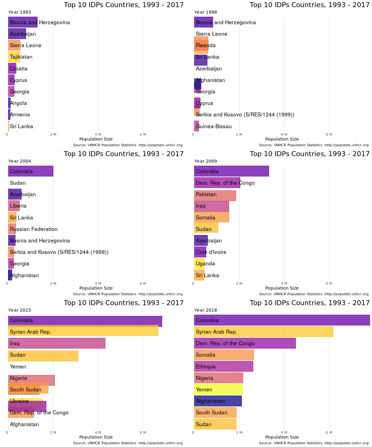
anim_save("bar_chart_race_refugee.gif", animate(p, fps = 1, nframes = 250, end_pause = 20, width = 600))

the same bar chart race but for IDPs..

p <- ggplot(rank_data2[rank_data2$Population.type %in% c("Internally displaced persons"), ]) +
  geom_bar(aes(y = Value2,  x =   reorder(ordering, desc(ordering)),
               group = Country ,color = Country, fill = Country), alpha = 0.75, stat = "identity") +
  
  geom_label(aes(y = 0 , x =  reorder(ordering, desc(ordering)), label = Country),
             hjust = 0,
             vjust = 0.5,
             fill = NA,
             label.size = NA,
             family = "Helvetica",
             size = 6) +
  
  coord_flip(clip = "off", expand = FALSE) +
  scale_color_viridis_d(option = "plasma" ) +
  scale_fill_viridis_d(option = "plasma") +
  scale_y_continuous(labels = format_si()) +
  theme_minimal(14, "Avenir") +
  #facet_wrap( ~ Population.type) +
  #facet_grid(. ~ Population.type) +
  
  ## get the animation per year... #, nframes = 250, fps = 10, end_pause = 20
  transition_time(Year ) +
  ease_aes('cubic-in-out') + 
 # enter_fade() +
 # exit_fade() +
  #view_follow(fixed_y = TRUE) +
  
  guides(color = F, fill = F) +
  labs(title =  "Top 10 IDPs Countries, 1993 - 2017",
       subtitle = 'Year {frame_time}',
       y = "Population Size",
       x = "",
       caption =  "Source: UNHCR Population Statistics -http://popstats.unhcr.org ") +
  theme(plot.title = element_text(hjust = 1, size = 22),
        axis.ticks.y = element_blank(),
        axis.text.y  = element_blank(), 
        panel.background  = element_blank(), 
        panel.grid = element_blank(),
        plot.background = element_blank(),
        legend.position = "bottom",
        panel.grid.major.x = element_line(color = "#cbcbcb"), 
        panel.grid.major.y = element_blank()) 

#animate(p, nframes = 250, fps = 4, end_pause = 20, width = 600)
animate(p, fps = 1, nframes = 250, end_pause = 20, width = 600)

anim_save("bar_chart_race_idp.gif", animate(p, fps = 1, nframes = 250, end_pause = 20, width = 600))

post

Home

About

Contributors

Categories

Join the Skype-group

learn more with R-bloggers

Recent posts

Anonymisation: Intrusion scenario and risk threshold

Post

Working with Survey Samples in the Tidyverse

Using Gridded Population Data for Household Survey Sampling

Quick tips for visualising data (with R)

Conjoint analysis: modeling judgement to calibrate vulnerability scoring

Using Analytic Hierarchy Process to weight vulnerability scorecard