This example is based on the note: A new index of refugee protection. It explainss the construction of a lack-of-protection index (or “index of protection risks”), a composite indicator constructed from two sub-dimensions: safety problems (18 indicators) and movement restrictions (6 indicators). To feel safe and secure in one’s home and surroundings is one of the core aspects of humanitarian protection, as is the freedom of movement.
The Limitation of measurement based on incident analysis
It is tempting to build measures of protection or of the lack thereof from counts of incident sand of other reported events for populations at risk. Incidents reveal major underlying problems. However, incidence rates are often so low, incomplete or unreliable that they frustrate robust measures. Additionally, incident reporting quality varies greatly due to differences in camp management across the settlements.
Incident counts discriminate well between a small number of communities at elevated risk and the vast majority at lesser risk. However, whether a municipality suffered “at least one incident in the past” vs “none ever” is extremely random. Statistical models for dealing with these kinds of rare events are available from the disease surveillance field. The major challenges are:
The signal-to-noise ratio is low, i.e. the detection of incident patterns is hampered by numerous random events and measurement errors.
The optimal density of the monitoring network is hard to determine. Too few observation points miss out on local structure; too many produce low counts per point(many with zeros), which makes the modeling and estimation difficult.
From a practical view point, one can either get fast results with many false positives, or more reliable measurements with delayed detection of true epidemics.
An alternative to incident-based statistics seems desirable. Such approach would potentially circumnavigate one of the major problems with using protection monitoring data (in addition to sensitivity and anonymity) – that incident reporting does not adequately reflect the pattern of protection challenges.
Using Betti-Verma weighting scheme
One of the many statistical methods for generating indicator weights and calculating sub-indices is known as the “Betti-Verma weighting scheme” or BV method. Betti and Verma(1999) and later others developed it for the measurement of deprivation (of individuals and households) in the field of poverty research. Betti-Verma determines indicator weights on the basis of two sets of statistical relationships: 1. The correlation pattern; the larger the sum of the coefficients with all theother variables, the more redundant is the indicator in point, and the smaller tends to be its weight; 2. The coefficient of variation, with indicators with higher coefficients getting higher weights.
“Betti-Verma weighting scheme” has an ability to deal with large numbers of indicators. Indicator datasets often include subsets of indicators that are highly correlated. This happens, for example, when sub populations all experience the same phenomena. The Betti-Verma method detects redundancy among indicators, reducing the weights on those that are strongly correlated with others. It calculates weights on indicators that contribute to a sub-index or index of interest. It increases the weights of indicators that are more informative (technically: have a larger coefficient of variation) and decreases weights of indicators that are more redundant (have larger correlations with all the other indicators). Both mechanisms reward diversity, the novel information that a particular indicator provides. This allows indices to include multiple correlated indicators and to avoid bias against others of equal substantive importance, but which are less strongly correlated.
The major strength of this method is to avoid “apples and oranges” issues in aggregation. It determines weights solely on the basis of the information contributions of the indicators. Betti-Verma weights are not substantive importance weights; the method throws a wide net to capture aspects of the concept of interest that are not yet covered in the statistical correlation patterns of the other indicators. A simplified technical explanation may be found in Composite measures of local disaster impact -Lessons from Typhoon Yolanda, Philippines
Its major weakness is that the method rewards measurement error. If a participating variable is measured with substantial error, its correlations with other, more reliablevariables are diminished fro m their true values. A lower sum of posit ive correlat ioncoefficients, however, increases the weight of the variable because it makes it appear to contribute more novel information.
Finally, contrary to methods that emphasize a narrow focus (scales, factor analysis), Betti-Verma, with its premium on diversity of deprivation aspects, has no ready reliability tests(e.g., no analogue to Cronbach’s Alpha). This is outweighed by the ability to reduce doubts and disputes over the relative importance of the indicators within a sector.
Package and functions required for the analysis
A new package
knitr::opts_chunk$set(
 collapse = TRUE,
 comment = " "
)
## This function will retrieve the packae if they are not yet installed.
using <- function(...) {
    libs <- unlist(list(...))
    req <- unlist(lapply(libs,require,character.only = TRUE))
    need <- libs[req == FALSE]
    if (length(need) > 0) {
        install.packages(need)
        lapply(need,require,character.only = TRUE)
    }
}

## Getting all necessary package
using("readxl", "httr", "tidyverse", "qvcalc","kableExtra","cluster","ClustOfVar","dendextend",
      "moments","sjstats","sp","ape","spdep","ncf", "spatstat","tmap","tmaptools",
                     "ggthemes", "ggrepel", "GGally", "ggpubr")

rm(using)

# install package devtools if not yet installed
# install.packages("devtools")
# install fast from GitHub without vignettes (not recommanded)
# devtools::install_github("a-benini/mdepriv")
library(mdepriv)

## Function used to scale variables from 0 to 1
range01 <- function(x){(x - min(x))/(max(x) - min(x))}

## Style to apply to ggplot2
unhcr_style <- function() {
  font <- "Lato"
  ggplot2::theme(

#This sets the font, size, type and colour of text for the chart's title
  plot.title = ggplot2::element_text(family = font, size = 13, face = "bold", color = "#222222"),

#This sets the font, size, type and colour of text for the chart's subtitle,  as well as setting a margin between the title and the subtitle
  plot.subtitle = ggplot2::element_text(family = font, size = 11, margin = ggplot2::margin(9,0,9,0)),
  plot.caption = ggplot2::element_blank(),

#This sets the position and alignment of the legend, removes a title and backround for it and sets the requirements for any text within the legend. The legend may often need some more manual tweaking when it comes to its exact position based on the plot coordinates.
  legend.position = "top",
  legend.text.align = 0,
  legend.background = ggplot2::element_blank(),
  legend.title = ggplot2::element_blank(),
  legend.key = ggplot2::element_blank(),
  legend.text = ggplot2::element_text(family = font, size = 13, color = "#222222"),

#This sets the text font, size and colour for the axis test, as well as setting the margins and removes lines and ticks. In some cases, axis lines and axis ticks are things we would want to have in the chart
  axis.title = ggplot2::element_blank(),
  axis.text = ggplot2::element_text(family = font, size = 13, color = "#222222"),
  axis.text.x = ggplot2::element_text(margin = ggplot2::margin(5, b = 10)),
  axis.ticks = ggplot2::element_blank(),
  axis.line = ggplot2::element_blank(),

#This removes all minor gridlines and adds major y gridlines. In many cases you will want to change this to remove y gridlines and add x gridlines.
  panel.grid.minor = ggplot2::element_blank(),
  panel.grid.major.y = ggplot2::element_line(color = "#cbcbcb"),
  panel.grid.major.x = ggplot2::element_blank(),

#This sets the panel background as blank, removing the standard grey ggplot background colour from the plot
  panel.background = ggplot2::element_blank(),

#This sets the panel background for facet-wrapped plots to white, removing the standard grey ggplot background colour and sets the title size of the facet-wrap title to font size 22
  strip.background = ggplot2::element_rect(fill = "white"),
  strip.text = ggplot2::element_text(size  = 13,  hjust = 0)
  )
}

# This small function is used to have nicely left align text within charts produced with ggplot2
left_align <- function(plot_name, pieces){
  grob <- ggplot2::ggplotGrob(plot_name)
  n <- length(pieces)
  grob$layout$l[grob$layout$name %in% pieces] <- 2
  return(grob)
}
Data used for analysis
Data used for the analysis is the IOM Bangladesh - Needs and Population Monitoring (NPM) Round 9 Site Assessment of the Rohingya Refugee Camps in Bangladesh, from March 2018, available in HDX
url1 <- "https://data.humdata.org/dataset/bef9f529-5ec0-4b31-a1fb-e9cb2eb1c987/resource/db78b145-eace-4113-a095-c63cbc9fd67f/download/npm-r9-site-assessment-dataset_2018-03-25.xlsx"

# GET(url1, write_disk(tf <- tempfile(fileext = ".xlsx")))
# data <- readxl::read_excel(tf, sheet = "Dataset")

#download.file(url1, destfile = "npm-r9-site-assessment-dataset_2018-03-25.xlsx" )
data <- readxl::read_excel("npm-r9-site-assessment-dataset_2018-03-25.xlsx", sheet = "Dataset")
#class(data)
## Force object to be a data frame
data <- as.data.frame(data)


## Rename variables of interest for the rest of the analysis so that they looks better in charts
data$Safe_Bathing_Child <- data$Children_safety_problems_Bathing_washing_facility
data$Safe_Market_Child <- data$Children_safety_problems_Market
data$Safe_Transportation_Child <- data$Children_safety_problems_Transportation
data$Safe_Waterpoints_Child <- data$Children_safety_problems_Waterpoints
data$Safe_Distribution_Child <- data$Children_safety_problems_Distribution_site
data$Safe_Firewood_Child <- data$Children_safety_problems_Firewood_collection_point
data$Safe_Bathing_Female <- data$Female_safety_problems_Bathing_washing_facility
data$Safe_Market_Female <- data$Female_safety_problems_Market
data$Safe_Transportation_Female <- data$Female_safety_problems_Transportation
data$Safe_Waterpoints_Female <- data$Female_safety_problems_Waterpoints
data$Safe_Distribution_Female <- data$Female_safety_problems_Distribution_site
data$Safe_Firewood_Female <- data$Female_safety_problems_Firewood_collection_point
data$Safe_Bathing_Male <- data$Male_safety_problems_Bathing_washing_facility
data$Safe_Market_Male <- data$Male_safety_problems_Market
data$Safe_Transportation_Male <- data$Male_safety_problems_Transportation
data$Safe_Waterpoints_Male <- data$Male_safety_problems_Waterpoints
data$Safe_Distribution_Male <- data$Male_safety_problems_Distribution_site
data$Safe_Firewood_Male <- data$Male_safety_problems_Firewood_collection_point
data$Move_Work <- data$Movement_Restrictions_Going_to_work
data$Move_Market <- data$Movement_Restrictions_Going_to_market
data$Move_Distribution <- data$Movement_Restrictions_At_distribution_site
data$Move_Firewood <- data$Movement_Restrictions_Collecting_firewood
data$Move_Checkpoints <- data$Movement_Restrictions_Crossing_checkpoints
data$Move_betw_Camp <- data$Movement_Restrictions_Moving_from_one_camp_to_another

## Not used
#"Female_safety_problems_Prefer_not_to_answer",
#"Female_safety_problems_Dont_know",
#"Children_safety_problems_Prefer_not_to_answer",
#"Children_safety_problems_Dont_know",
#"Male_safety_problems_Prefer_not_to_answer",
#"Male_safety_problems_Dont_know")

#"Movement_Restrictions_Prefer_not_to_answer",
#"Movement_Restrictions_Dont_know"
Dimension
Dimension 1: Insecurity
First, we select and visualise variables of interest.
safety <- c("Safe_Bathing_Child",
            "Safe_Market_Child",
            "Safe_Transportation_Child",
            "Safe_Waterpoints_Child",
            "Safe_Distribution_Child",
            "Safe_Firewood_Child",
            "Safe_Bathing_Female",
            "Safe_Market_Female",
            "Safe_Transportation_Female",
            "Safe_Waterpoints_Female",
            "Safe_Distribution_Female",
            "Safe_Firewood_Female",
            "Safe_Bathing_Male",
            "Safe_Market_Male",
            "Safe_Transportation_Male",
            "Safe_Waterpoints_Male",
            "Safe_Distribution_Male",
            "Safe_Firewood_Male")

data %>%
  select(safety) %>%
  tidyr::gather(key = "item", value = "value") %>%
  ## note that we need to specify tidyr:: as gather function name is present in different packages
  ggplot(aes(value)) +
  geom_histogram(breaks = seq(0, 1, 0.05),stat = "count",colour = "white", fill = "#0072bc") +
  facet_wrap(~item, ncol = 3) +
  unhcr_style() +
  ggtitle("Items Distributions related to safety")
  Note: Using an external vector in selections is ambiguous.
  ℹ Use `all_of(safety)` instead of `safety` to silence this message.
  ℹ See <https://tidyselect.r-lib.org/reference/faq-external-vector.html>.
  This message is displayed once per session.
  Warning: Ignoring unknown parameters: binwidth, bins, pad, breaks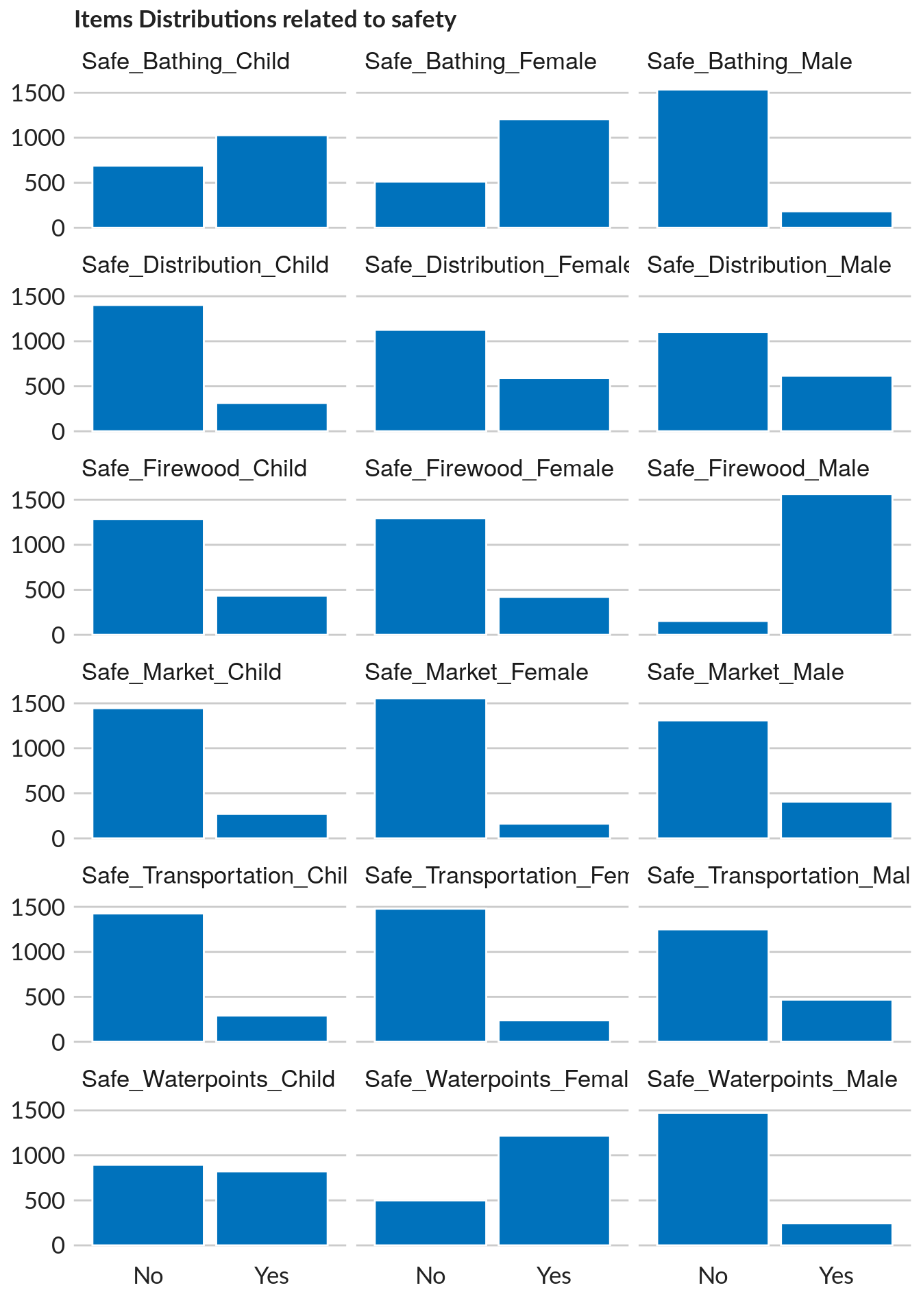
Then we check data structure in order to apply the model. We need to ensure that there’s no empty value and that all value are numeric. Additionally, values needs to be normalised from 0 to 1.
# all chosen safety items are characters and do not include any NA-values
data.frame(class = map_chr(data[ ,safety], ~class(.x)),
           anyNA = map_lgl(data[ ,safety], ~anyNA(.x)))
                                 class anyNA
  Safe_Bathing_Child         character FALSE
  Safe_Market_Child          character FALSE
  Safe_Transportation_Child  character FALSE
  Safe_Waterpoints_Child     character FALSE
  Safe_Distribution_Child    character FALSE
  Safe_Firewood_Child        character FALSE
  Safe_Bathing_Female        character FALSE
  Safe_Market_Female         character FALSE
  Safe_Transportation_Female character FALSE
  Safe_Waterpoints_Female    character FALSE
  Safe_Distribution_Female   character FALSE
  Safe_Firewood_Female       character FALSE
  Safe_Bathing_Male          character FALSE
  Safe_Market_Male           character FALSE
  Safe_Transportation_Male   character FALSE
  Safe_Waterpoints_Male      character FALSE
  Safe_Distribution_Male     character FALSE
  Safe_Firewood_Male         character FALSE

## We will need numeric value for the modeling phase - so
for (i in safety) {
 data[ ,i] = as.numeric(if_else(data[ ,i] == "Yes", 1L, 0L))
 }

# check if all safety items have become numeric ...
map_chr(data[ ,safety], ~class(.x)) %>% unique()
  [1] "numeric"
# ... yes they have

## Scale variables
#data[ , safety] <-  range01(data[ , safety])

#View(data[ , safety])
#str(data[ , safety])

## Count Number of NA
# cat("Count Number of NA within selected variables.\n")
# sapply(data[ , safety],function(x) sum(is.na(x)))
A cluster analysis of the variables reveals five of those six problems tend to co-occur closely (red rectangle in the dendrogram). The sixth - the safety problems that men face at relief distributions – aligns more closely with the same problem of women and children (orange rectangle) The safety of the three groups during transportation and market visits forms its own cluster, but the challenges for women and children (who may rarely move very far) and those for men (who likely do the shopping and travel in search for work) are not closely correlated. Some of this clustering could be a statistical artefact, caused by the individual propensities of key informants to check few or many problems.
# Create a dendrogram and plot it
dend <- data[ , safety] %>%
  #scale %>%
  #dist %>%
  hclustvar %>%
  as.dendrogram
dend <- dend %>% set("branches_k_color", k = 5)

# Rectangle dendrogram using ggplot2
ggd1 <- as.ggdend(dend)
#ggplot(ggd1)

dend1.plot <- ggplot(ggd1,
                     horiz = TRUE) +
  #scale_y_reverse()+
  theme_dendro() +
  #unhcr_style() +
  coord_flip() +
  labs(ylab = "Jacquard distance",
       title = "Clustering on Safety Variable ",
       subtitle = "",
       caption = "NPM Data")
  Coordinate system already present. Adding new coordinate system, which will replace the existing one.

ggpubr::ggarrange(left_align(dend1.plot, c("subtitle", "title", "caption")), ncol = 1, nrow = 1)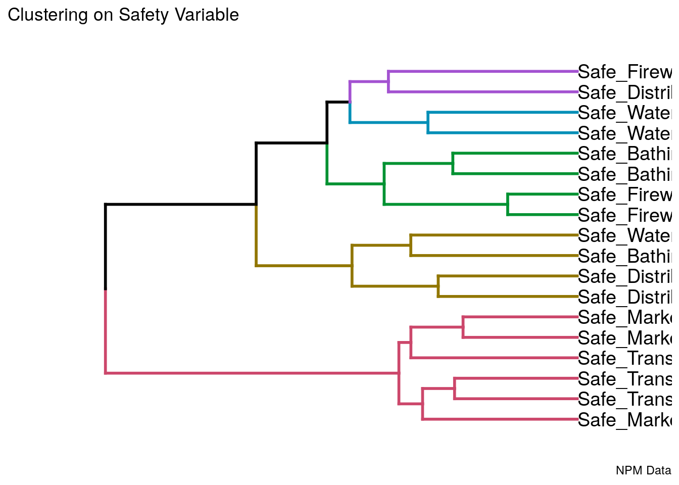
Dimension 2: movement restrictions
The correlation pattern among the six indicators has two abnormalities – a medium strong negative correlation between movement restrictions on the way to work and at distribution sites, and a perfect positive correlation between restrictions at checkpoints and atdistribut ions sites. The former may indicate different safet y profiles for populat ion wit hgreater and lesser integration into local job markets. The second, seen in this cross-tabulation is more of an enigma: It implies that friendly checkpoints go hand in hand with safe movement to and fromdistribution sites, but not the reverse. The 74 camp points with zeros in both indicators reveal either an interesting protection regularity or a data management problem, using zerosinappropriately for missing values. Which it is only research on the ground will tell. The dendrogram reflects stronger coincidences among restrictions experienced while going to work, at checkpoints and while collecting firewood. Interestingly, although restrictions at checkpoints and at distribution sites are perfectly correlated, “at distribution sites” has moved away.
movement <- c("Move_Work",
            "Move_Market",
            "Move_Distribution",
            "Move_Firewood",
            "Move_Checkpoints",
            "Move_betw_Camp")

data %>%
  select(movement) %>%
  tidyr::gather(key = "item", value = "value") %>%
  ## note that we need to specify tidyr:: as gather function name is present in different packages
  ggplot(aes(value)) +
  geom_histogram(breaks = seq(0, 1, 0.05),stat = "count",colour = "white", fill = "#0072bc") +
  facet_wrap(~item, ncol = 2) +
  unhcr_style() +
  ggtitle("Items Distributions related to Movement")
  Note: Using an external vector in selections is ambiguous.
  ℹ Use `all_of(movement)` instead of `movement` to silence this message.
  ℹ See <https://tidyselect.r-lib.org/reference/faq-external-vector.html>.
  This message is displayed once per session.
  Warning: Ignoring unknown parameters: binwidth, bins, pad, breaks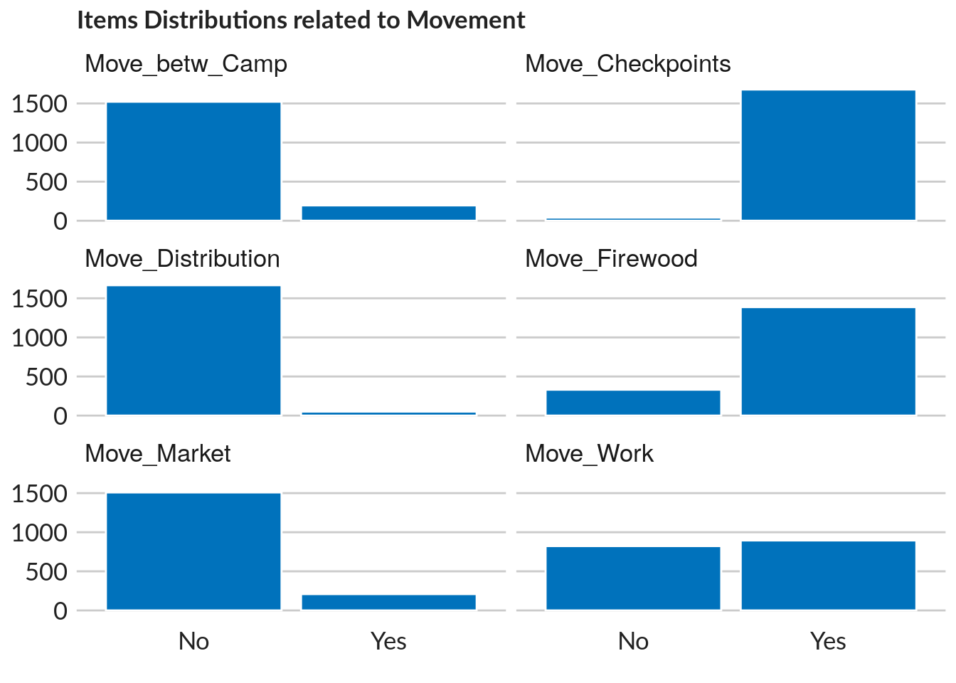
Then we check data structure in order to apply the model. We need to ensure that there’s no empty value and that all value are numeric. Additionally, values needs to be normalised from 0 to 1.
# all chosen safety items are characters and do not include any NA-values
data.frame(class = map_chr(data[ ,movement], ~class(.x)),
           anyNA = map_lgl(data[ ,movement], ~anyNA(.x)))
                        class anyNA
  Move_Work         character FALSE
  Move_Market       character FALSE
  Move_Distribution character FALSE
  Move_Firewood     character FALSE
  Move_Checkpoints  character FALSE
  Move_betw_Camp    character FALSE

## We will need numeric value for the modeling phase - so
for (i in movement) {
 data[ ,i] = as.numeric(if_else(data[ ,i] == "Yes", 1L, 0L))
 }

# check if all movement items have become numeric ...
map_chr(data[ ,movement], ~class(.x)) %>% unique()
  [1] "numeric"
# ... yes they have

## Scale variables
#data[ , movement] <-  range01(data[ , movement])

#View(data[ , movement])
#str(data[ , movement])

## Count Number of NA
# cat("Count Number of NA within selected variables.\n")
# sapply(data[ , movement],function(x) sum(is.na(x)))
Again, we apply a variable cluster analysis.
# Create a dendrogram and plot it
dend <- data[ , movement] %>%
  #scale %>%
  #dist %>%
  hclustvar %>%
  as.dendrogram
dend <- dend %>% set("branches_k_color", k = 3)

# Rectangle dendrogram using ggplot2
ggd1 <- as.ggdend(dend)
#ggplot(ggd1)
#ggplot(ggd1)

dend1.plot <- ggplot(ggd1,
                     horiz = TRUE) +
  #scale_y_reverse()+
  theme_dendro() +
  #coord_flip() +
  #unhcr_style() +
  #coord_cartesian( clip = 'off') +   # This keeps the labels from disappearing
  theme(plot.margin = unit(c(1,2,1,1),"cm")) +# top, right, bottom, left
  #theme(plot.margin = unit(c(t = 0, r = 10, b = 0, l = 0), unit = "pt")) +
  #theme(plot.margin = unit(c(1, 4, 1, 1), "pt")) +

  labs(ylab = "Jacquard distance",
       title = "Clustering on Movement Variable ",
       subtitle = "",
       caption = "NPM Data")

ggpubr::ggarrange(left_align(dend1.plot, c("subtitle", "title", "caption")), ncol = 1, nrow = 1)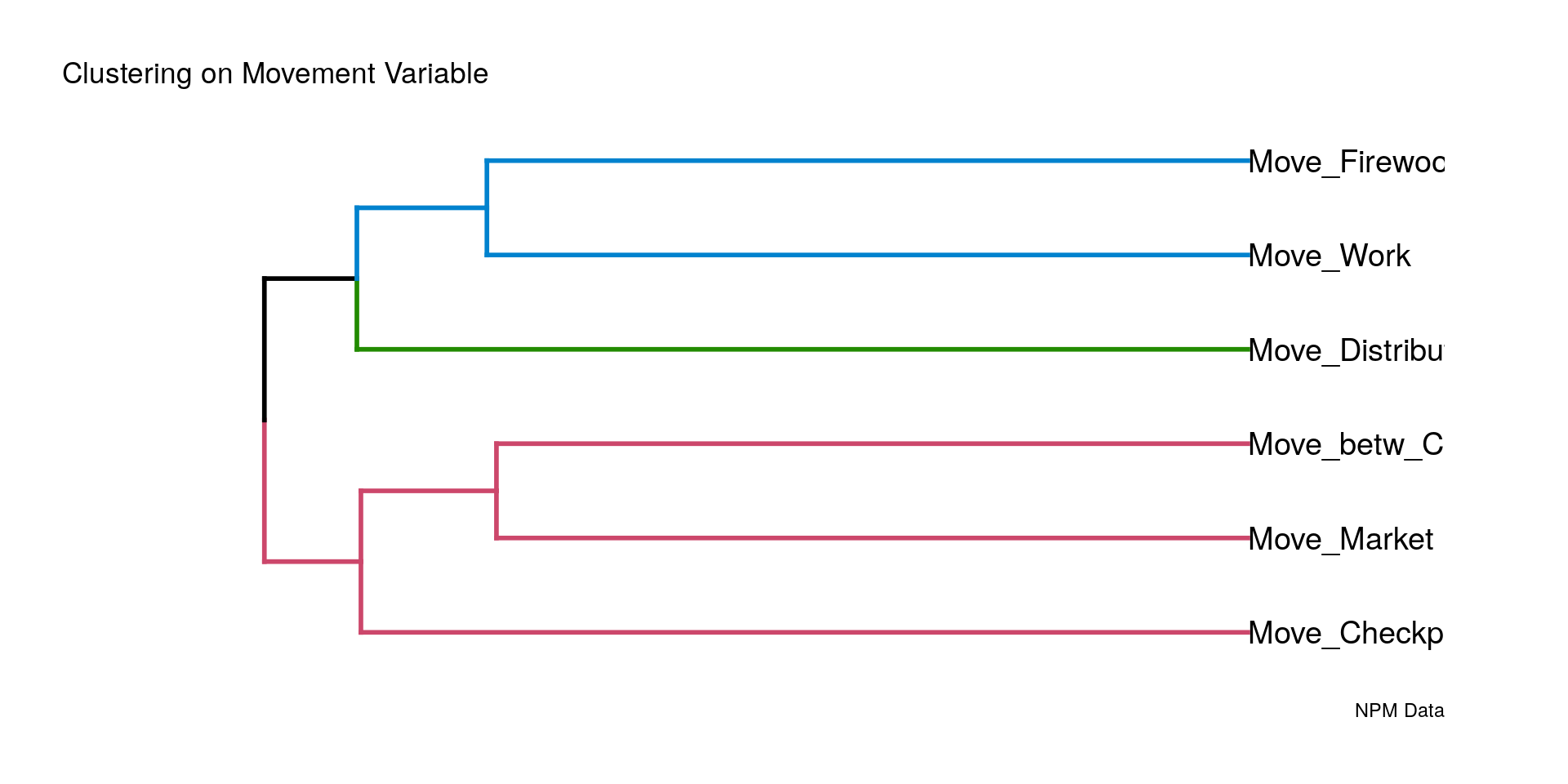
Running the model
Items & Dimensions weight
#summary(data[ , c(movement,safety)])
model_1 <- mdepriv(data,
                   items = list('safety' = safety,
                                   'movement' = movement), # 2nd argument items in a named list grouped
                   method = "bv",
                   output = "all")
# get all possible outputs/returns -> select later on required elements s. below- The “Index” column gives the proportions of refugees for which a particular safety problem was reported (the population-weighted prevalence among camp points).
- The weights are those used in the aggregation.
- The contributions are the prevalences multiplied by their weights; they represent the indicators’ contributions to the sub-index.
- The shares, summed to 1,make it easier to compare the contributions.
kable(model_1$summary_by_dimension,
       caption = "Summary by dimension") %>%
kable_styling(bootstrap_options = c("striped", "bordered", "condensed", "responsive"), font_size = 9)| Dimension | N_Item | Index | Weight | Contri | Share |
|---|---|---|---|---|---|
| movement | 18 | 0.1861321 | 0.5 | 0.0930661 | 0.3733313 |
| safety | 6 | 0.3124387 | 0.5 | 0.1562194 | 0.6266687 |
| Total | 24 | NA | 1.0 | 0.2492854 | 1.0000000 |
kable(model_1$summary_by_item,
       caption = "Summary by item") %>%
kable_styling(bootstrap_options = c("striped", "bordered", "condensed", "responsive"), font_size = 9)| Dimension | Item | Index | Weight | Contri | Share |
|---|---|---|---|---|---|
| safety | Safe_Bathing_Child | 0.5983702 | 0.0213341 | 0.0127657 | 0.0512092 |
| safety | Safe_Market_Child | 0.1583236 | 0.0137107 | 0.0021707 | 0.0087078 |
| safety | Safe_Transportation_Child | 0.1699651 | 0.0178266 | 0.0030299 | 0.0121544 |
| safety | Safe_Waterpoints_Child | 0.4784633 | 0.0129588 | 0.0062003 | 0.0248723 |
| safety | Safe_Distribution_Child | 0.1833527 | 0.0136681 | 0.0025061 | 0.0100531 |
| safety | Safe_Firewood_Child | 0.2526193 | 0.0274911 | 0.0069448 | 0.0278587 |
| safety | Safe_Bathing_Female | 0.7019790 | 0.0077932 | 0.0054707 | 0.0219453 |
| safety | Safe_Market_Female | 0.0948778 | 0.0157384 | 0.0014932 | 0.0059900 |
| safety | Safe_Transportation_Female | 0.1391153 | 0.0141243 | 0.0019649 | 0.0078822 |
| safety | Safe_Waterpoints_Female | 0.7089639 | 0.0133591 | 0.0094711 | 0.0379931 |
| safety | Safe_Distribution_Female | 0.3440047 | 0.0138082 | 0.0047501 | 0.0190548 |
| safety | Safe_Firewood_Female | 0.2456345 | 0.0459441 | 0.0112855 | 0.0452712 |
| safety | Safe_Bathing_Male | 0.1065192 | 0.0272135 | 0.0028988 | 0.0116283 |
| safety | Safe_Market_Male | 0.2374854 | 0.0129966 | 0.0030865 | 0.0123814 |
| safety | Safe_Transportation_Male | 0.2729919 | 0.0098239 | 0.0026818 | 0.0107581 |
| safety | Safe_Waterpoints_Male | 0.1426077 | 0.0258954 | 0.0036929 | 0.0148139 |
| safety | Safe_Distribution_Male | 0.3591385 | 0.2032094 | 0.0729803 | 0.2927581 |
| safety | Safe_Firewood_Male | 0.9103609 | 0.0031044 | 0.0028261 | 0.0113368 |
| movement | Move_Work | 0.5209546 | 0.0542091 | 0.0282405 | 0.1132857 |
| movement | Move_Market | 0.1216531 | 0.0744375 | 0.0090556 | 0.0363260 |
| movement | Move_Distribution | 0.0296857 | 0.2059834 | 0.0061148 | 0.0245291 |
| movement | Move_Firewood | 0.8073341 | 0.0150103 | 0.0121183 | 0.0486121 |
| movement | Move_Checkpoints | 0.9767171 | 0.0236289 | 0.0230788 | 0.0925796 |
| movement | Move_betw_Camp | 0.1140861 | 0.1267308 | 0.0144582 | 0.0579987 |
| Total | NA | NA | 1.0000000 | 0.2492854 | 1.0000000 |
Histogram of the insecurity subindex
The Coefficient of variation is a measure of relative dispersion representing the degree of variability relative to the mean
Skewness and kurtosis measurement allows to confirm whether the scores distribution is “normal”.
Skewness assesses the extent to which a variable’s distribution is symmetrical (degree of distortion). If the distribution of responses for a variable stretches toward the right or left tail of the distribution, then the distribution is referred to as skewed. A general guideline for skewness is that if the number is greater than +1 or lower than –1, this is an indication of a substantially skewed distribution.
Kurtosis is a measure of whether the distribution is too peaked (a very narrow distribution with most of the responses in the center). it is actually a measure of outliers. For kurtosis, the general guideline is that if the number is greater than +3, the distribution is too peaked. Likewise, a kurtosis of less than –3 indicates a distribution that is too flat.
We can check each dimension and the aggregated score.
data$move_scores <- mdepriv(data,
                     method = "bv",
                      items <- list('movement' <- movement),
                     output = "score_i")

# Chart
histo <-  ggplot(data, aes(move_scores)) +
    geom_histogram(bins = 10,  colour = "white", fill = "#0072bc") +
    geom_hline(yintercept = 0, size = 1, colour = "#333333") +
    unhcr_style() +
    labs(ylab = "Unique Block",
         title = "Distribution of Refugee Movement Deprivation Sub-Index",
         subtitle = paste0("Mean: ",round(mean(data$move_scores),2) ,
                           ", Standard Deviation: ",round(sd(data$move_scores),2) ,
                           ", Coefficient of Variation: ",round(cv(data$move_scores),2) ,
                           ", Skewness: ",round(skewness(data$move_scores),2) ,
                           " and Kurtosis: ",round(kurtosis(data$move_scores),2) ),
         caption = "NPM Data")

ggpubr::ggarrange(left_align(histo, c("subtitle", "title", "caption")), ncol = 1, nrow = 1)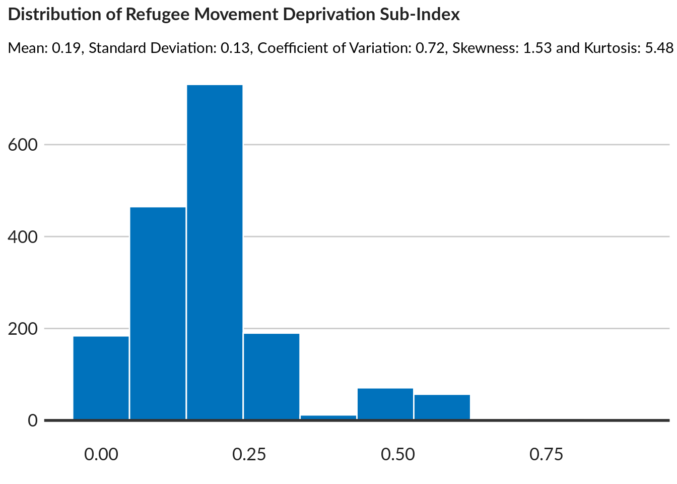
data$safe_scores <- mdepriv(data,
                     method = "bv",
                      items <- list('safety' <- safety),
                     output = "score_i")

# Chart
histo <-  ggplot(data, aes(safe_scores)) +
    geom_histogram(bins = 10, colour = "white", fill = "#0072bc") +
    geom_hline(yintercept = 0, size = 1, colour = "#333333") +
    unhcr_style() +
    labs(ylab = "Unique Block",
         title = "Distribution of Refugee Safety Deprivation  Sub-Index",
         subtitle = paste0("Mean: ",round(mean(data$safe_scores),2) ,
                           ", Standard Deviation: ",round(sd(data$safe_scores),2) ,
                           ", Coefficient of Variation: ",round(cv(data$safe_scores),2) ,
                           ", Skewness: ",round(skewness(data$safe_scores),2) ,
                           " and Kurtosis: ",round(kurtosis(data$safe_scores),2) ),
         caption = "NPM Data")

ggpubr::ggarrange(left_align(histo, c("subtitle", "title", "caption")), ncol = 1, nrow = 1)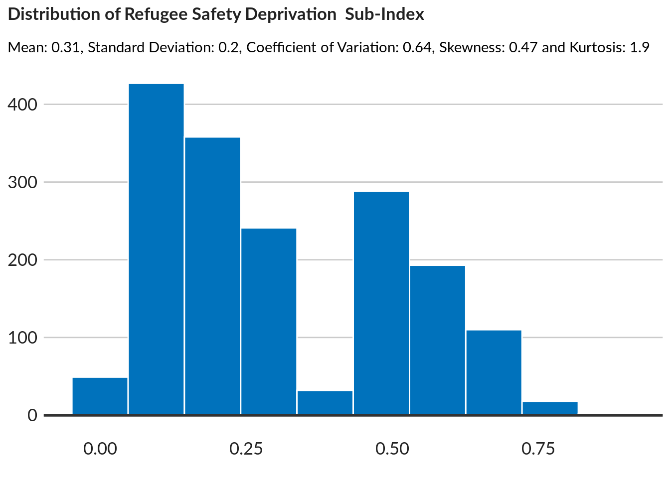
data$prot_scores <- mdepriv(data,
                    method = "bv",
                    items = list('safety' = safety,
                                   'movement' = movement),
                     output = "score_i")

# Chart
histo <-  ggplot(data, aes(prot_scores)) +
    geom_histogram(bins = 10, colour = "white", fill = "#0072bc") +
    geom_hline(yintercept = 0, size = 1, colour = "#333333") +
    unhcr_style() +
    labs(ylab = "Unique Block",
         title = "Distribution of Refugee Protection Deprivation Index",
         subtitle = paste0("Mean: ",round(mean(data$move_scores),2) ,
                           ", Standard Deviation: ",round(sd(data$prot_scores),2) ,
                           ", Coefficient of Variation: ",round(cv(data$prot_scores),2) ,
                           ", Skewness: ",round(skewness(data$prot_scores),2) ,
                           " and Kurtosis: ", round(kurtosis(data$prot_scores),2) ),
         caption = "NPM Data")

ggpubr::ggarrange(left_align(histo, c("subtitle", "title", "caption")), ncol = 1, nrow = 1)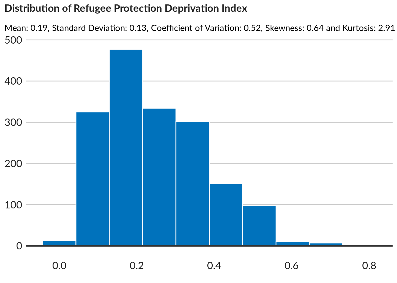
# Chart
histo <-  ggplot(data, aes(prot_scores)) +
    geom_histogram(bins = 10,  colour = "white", fill = "#0072bc") +
    geom_hline(yintercept = 0, size = 1, colour = "#333333") +
    unhcr_style() +
    facet_wrap(~ Union) +
    labs(ylab = "Unique Block",
         title = "Deprivation Index Level ",
         subtitle = "Distribution of Refugee Protection index",
         caption = "NPM Data")

ggpubr::ggarrange(left_align(histo, c("subtitle", "title", "caption")), ncol = 1, nrow = 1)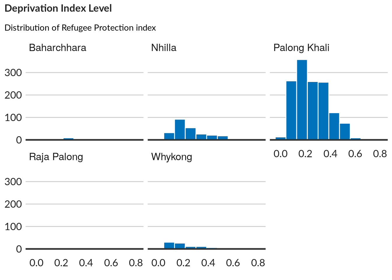
Distribution of the subindex in four areas (facet)
#
boxplot <-  ggplot(data, aes(x = Union, y = prot_scores, fill = `Site Type`  )) +
          stat_boxplot(geom = 'errorbar', width = 0.5, position = position_dodge(0.7)) +
          geom_boxplot(width = 0.6, position = position_dodge(0.7)) +
          unhcr_style() +
          scale_y_continuous(breaks = seq(0,1,0.2), limits = c(0,1)) +
          unhcr_style() +
    labs(ylab = "Unique Block",
         title = "Protection Deprivation Index ",
         subtitle = "Spread per Union & Location Type ",
         caption = "NPM Data") +
  theme(axis.text.x = element_text(angle = 45, hjust = 1))

ggpubr::ggarrange(left_align(boxplot, c("subtitle", "title", "caption")), ncol = 1, nrow = 1)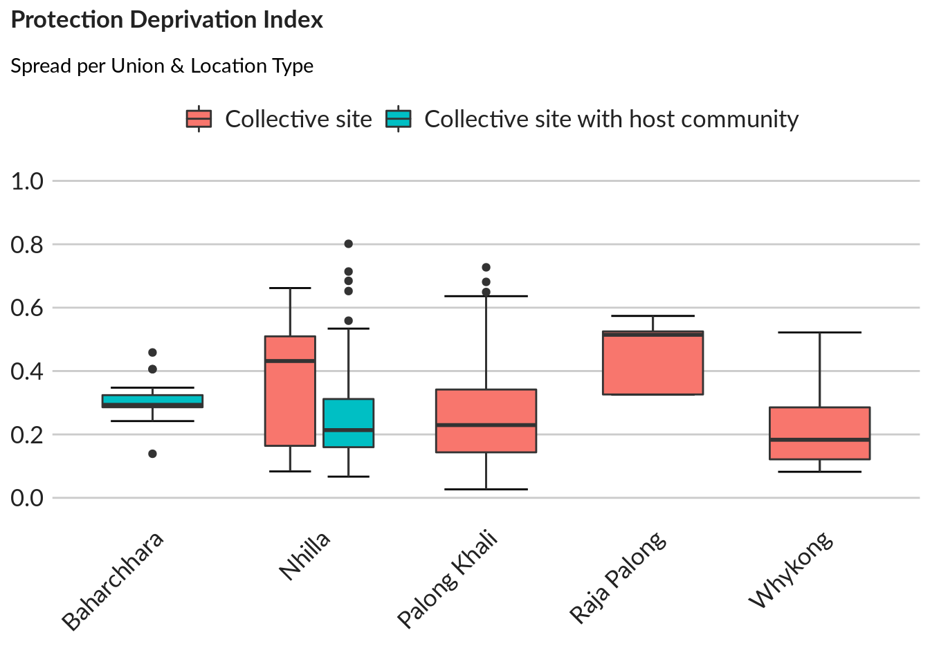
Spatial Correlation: identification of hotspots
data$Lon <- data$"_Geopoint_longitude"
data$Lat <- data$"_Geopoint_latitude"
data$total <- data$"Total HH"

xy <- data[,c( "Lon","Lat" )]

SPDF <- SpatialPointsDataFrame(coords = xy, data = data,
                               proj4string = CRS("+proj=longlat +datum=WGS84 +ellps=WGS84 +towgs84=0,0,0"))

#  [12] "Total HH"
# [13] "Total Ind"
SPDF.K <- SPDF[ SPDF$Union == "Palong Khali", ]
SPDF.K_sf <- st_as_sf(SPDF.K,
                       coords = c("Lon", "Lat"),
                       crs = 4326)
tmap::tmap_mode("plot")
  tmap mode set to plotting
## tmap style set
tmap::tmap_style("white")
  tmap style set to "white"
  other available styles are: "gray", "natural", "cobalt", "col_blind", "albatross", "beaver", "bw", "classic", "watercolor"
## other available styles are: "white", "gray", "natural", "cobalt", "col_blind",
#"albatross", "beaver", "bw", "watercolor"

# plot with regular tmap functions
#tm_shape(osm_tile) +
tm_shape(SPDF.K_sf) +
tm_bubbles(col = "prot_scores",
           size = "total",
           border.col = "white",
           border.lwd = 1,
           #shape = 21,
           alpha = 0.8,
           n = 5,  #number of color scale classes
           style = "pretty", #method to process the color scale
           palette = "viridis",
           scale = 0.85,
           legend.max.symbol.size = 1,
           title = "Index in relation to population",
           title.size = "Total HH",
           legend.size.is.portrait  = TRUE,
           title.col = "Protection Score",
           legend.col.is.portrait  = TRUE) +
tm_legend(outside = TRUE,
          outside.position = "right",
          stack = "vertical")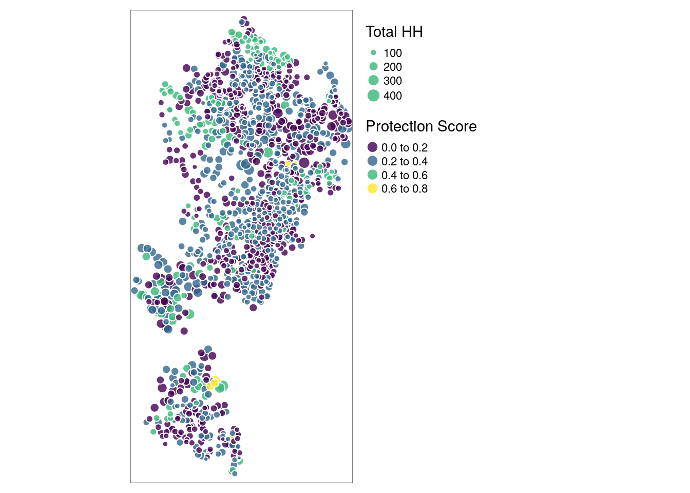
Moran’s I is a well-known test for spatial autocorrelation. It is a particular case of the general cross-product that depends on a spatial weight matrix or a distance related decline function. Like a correlation coefficient, the values of Moran’s I range from +1 meaning strong positive spatial autocorrelation to 0 meaning a random pattern to -1 indicating strong negative spatial autocorrelation. The Spatial Autocorrelation with Global Moran’s I is an inferential statistic, which means that the results of the analysis are always interpreted within the context of its null hypothesis.
We first need to compute the neighbourhood matrix dist.w
data.dists <- as.matrix(dist(cbind(data$Lon, data$Lat)))
data.dists.inv <- 1/data.dists
diag(data.dists.inv) <- 0
dist.w <- mat2listw(data.dists.inv)
We can now compute the Moran’s I indicator it with Monte Carlo simulation.
# Moran with ape package
# moran.prot <- ape::Moran.I(data$prot_scores, data.dists.inv)
# cat(paste0("Moran's test for Protection deprivation p-value is ",moran.prot$p.value, "\n" ))
#
# moran.move <- ape::Moran.I(data$move_scores, data.dists.inv)
# cat(paste0("Moran's test for Movement deprivation p-value is ",moran.move$p.value, "\n" ))
#
# moran.safe <- ape::Moran.I(data$safe_scores, data.dists.inv)
# cat(paste0("Moran's test for Safetyn deprivation p-value is ",moran.safe$p.value, "\n" ))

# Moran without Monte Carlo
# moran.test(data$prot_scores,
#            dist.w )

# Moran with Monte Carlo


moran.mc(data$move_scores,
         dist.w,
         nsim = 99,
         zero.policy = T)

    Monte-Carlo simulation of Moran I

  data:  data$move_scores
  weights: dist.w
  number of simulations + 1: 100

  statistic = 0.065441, observed rank = 100, p-value = 0.01
  alternative hypothesis: greater


moran.mc(data$safe_scores,
         dist.w,
         nsim = 99,
         zero.policy = T)

    Monte-Carlo simulation of Moran I

  data:  data$safe_scores
  weights: dist.w
  number of simulations + 1: 100

  statistic = 0.037278, observed rank = 100, p-value = 0.01
  alternative hypothesis: greater


moran.mc(data$prot_scores,
         dist.w,
         nsim = 99,
         zero.policy = T)

    Monte-Carlo simulation of Moran I

  data:  data$prot_scores
  weights: dist.w
  number of simulations + 1: 100

  statistic = 0.043762, observed rank = 100, p-value = 0.01
  alternative hypothesis: greater
The spatial correlation of the movement restriction sub-index is stronger than that of insecurity. This applies particularly to within-camp situations and to neighboring points across the border of two camps. It means that neighboring points tend to both have either higher sub-index values, or both of them lower ones.
We can finally test how much the Protection Deprivation Index is spatially correlated in terms of distance.
## First we need to reproject the Spatial Point dataframe to a CRS that allows calculation in meters.
## WGS 84 / UTM zone 45N - CRS is 32645 -- CRS("+init=epsg:32645")

SPDF.32645 <- spTransform(SPDF,"+init=epsg:32645" )


# leadI <- ncf::spline.correlog(x=data$Lon, y=data$Lat,
#                          z=data$prot_scores,
#                          resamp = 100, quiet=TRUE)

leadI <- ncf::spline.correlog(x = coordinates(SPDF.32645)[,1],
                              y = coordinates(SPDF.32645)[,2],
                              z = SPDF.32645$prot_scores,
                              resamp = 100,
                              quiet = TRUE)

plot(leadI, main = "Spatial autocorrelation in relation to distance")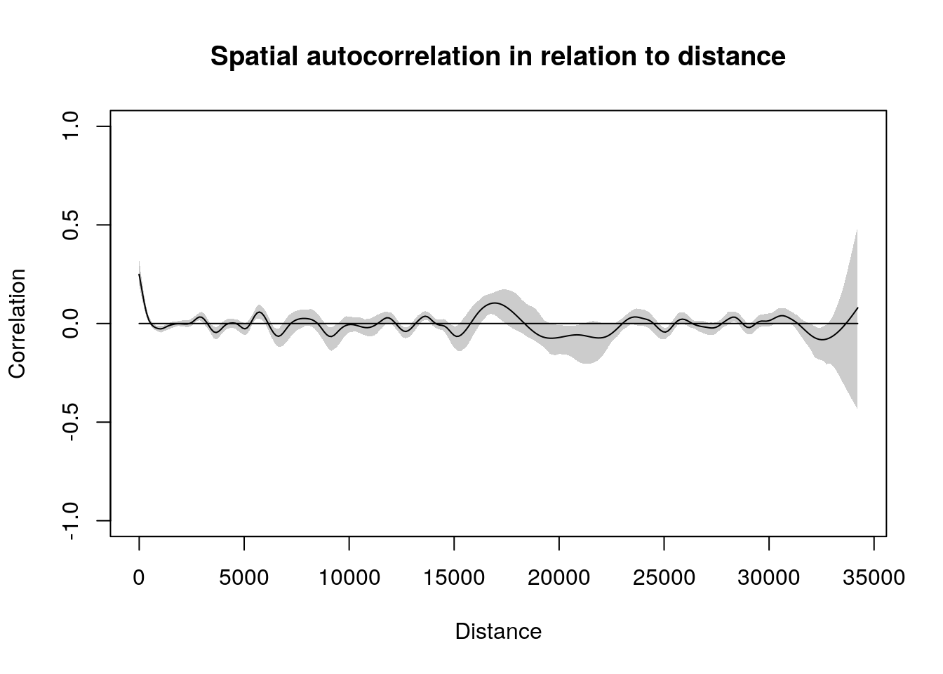
Discussion on index properties
The sub-indices are similar in mean and standard deviation (SD), and their skewness (a measure of asymmetry) is close to that of a normal distribut ion (0). The same for their kurtosis (a measure of thin or thick tails; the kurtosis of a normal distribution is 3).Neither are there any missing values (both sub-indices cover the full population). Moreover,since for every sub-index Betti-Verma sets the sum of weights on the indicators = 1, the means are directly comparable. In sum, these two constructs seem formally well-behaved.
Properties of the subindices need to be noted:
Measurement level: The sub-indices, differently from the indicators, are no longer merely binary; they are ratio-level with multiple distinct values. The ratio-level characterization is reasonable if we think that a zero value signifies the absence of insecurity, respectively movement restrictions.
Information value: Ratio-level sub-indices are more informative when their variablility, measured by the coefficients of variation (= standard deviation divided by the mean) is larger.
The correlation between the sub-indices: Since they are at ratio-level constructs, the Pearson correlation is appropriate.
The two sub-indices are weakly positively correlated. This might be counter intuitive: why would refugees subjected to more movement restrictions not feel more insecure? A potential explanation is that the conditions on the ground responsible for insecurity, respectively for movement restrictions are fairly independent the ones from the others. Speculatively, we can invoke two hypothesis that could explain the low correlation:
First, security may be better where the Bangladeshi military are maintaining a stronger presence. A stronger presence implies more stringent checkpoints. The coincidence in some places of better security and tighter movement restrictions would dampen the overall correlation.
Second, the two sub-indices describe very different problems. If so, it may be necessaryto rethink the combination of protection variables altogether. One way to go about this would be to take the 6 – 8 most highly weighted (in Betti-Verma) insecurity and movement restrict ion indicators and statistically project them onto a multidimensional space, and then to study the distribution of camps over that space.
Share this post
Twitter
Google+
Facebook
Reddit
LinkedIn
StumbleUpon
Pinterest
Email