Often affected population or key informant are requested to share their preference for specific type of interventions. How can we identify patterns of preference within a dataset? Can we identify groupings on the basis of several (categorical or continuous) variables that differentiate profiles optimally.
This tutorial is based on the publication Priorities and preferences in humanitarian needs assessments -Their measurement by rating and ranking methods.
Loading packages
## This function will retrieve the packae if they are not yet installed.
using <- function(...) {
   libs <- unlist(list(...))
    req <- unlist(lapply(libs,require,character.only = TRUE))
    need <- libs[req == FALSE]
    if (length(need) > 0) {
        install.packages(need)
        lapply(need,require,character.only = TRUE)
    }
}

## Getting all necessary package
using("foreign", "PlackettLuce", "tidyverse", "qvcalc","kableExtra","stargazer","NLP",
                     "ggthemes", "ggrepel", "GGally", "bbplot","ggpubr",'grid','gridExtra', 'forcat', 'psychotree')
## [[1]]
## [1] FALSErm(using)
# This small function is used to have nicely left align text within charts produced with ggplot2
left_align <- function(plot_name, pieces){
grob <- ggplot2::ggplotGrob(plot_name)
n <- length(pieces)
grob$layout$l[grob$layout$name %in% pieces] <- 2
return(grob)
}Dataset
The data used in the this tutorial comes from NPM Site Assessment Round 11, 2018 - for the Rohingya refugee camps in Bangladesh.
data_csv <- read.csv(file = "181227_2027AB_NPM11_Priorities_PlackettLuce.csv", header = T, sep = ",")


used_var <- as.character(names(data_csv))[grepl("l_",as.character(names(data_csv)))]

# Structure of the data:
#str(data_csv)
Can we identify differences within preferences?
In the dataset, there are variables define groups among which sectoral needs priorities may differ significantly.This is corresponds to the detection of Differential Item Functioning (DIF).
For instance, we have 4 sub-districts with refugee settlements (upazila), a continuous population size variable for the 1,990 camp blocks (log10pop) (logarithmic), and the distance from the nearest health care facility (healthWalk_enc, with five levels) as a marginalization indicator. These
Rashtree Visualisation are designed to identify significant differences within preferences.
We first need to format the data so that it can be consumed by the algorithm.
covariate <- data_csv[, c("upazila", "log10pop", "healthWalk_enc")]

resp <- as.matrix(data_csv[, used_var])

## Rashtree accepts only 0 or 1 - so everything above 0 shalle be replaced by 1
for (i in 1:nrow(resp)) {
    for (j in 1:ncol(resp)) if (resp[i, j] > 0)
        resp[i, j] = 1
}
## resp will be a matrix variable used in the model
covariate$resp <- resp

# To exclude rows where all observed item responses are either 0 or 1, we select
# only the subsetof cases for which the proportion of correct item responses is
# strictly between 0 and 1 forfuther analysis.
covariate <- subset(covariate, rowMeans(resp, na.rm = TRUE) > 0 & rowMeans(resp,
    na.rm = TRUE) < 1)
We can now compute and display it.
If the Rasch tree shows at least one split, DIF is present and there are groups with significant difference in their hiearchy of needs.
## Compute the rashtree
raschtree <- raschtree(resp ~ upazila + log10pop + healthWalk_enc, data = covariate)

## and plotting it...
plot(raschtree)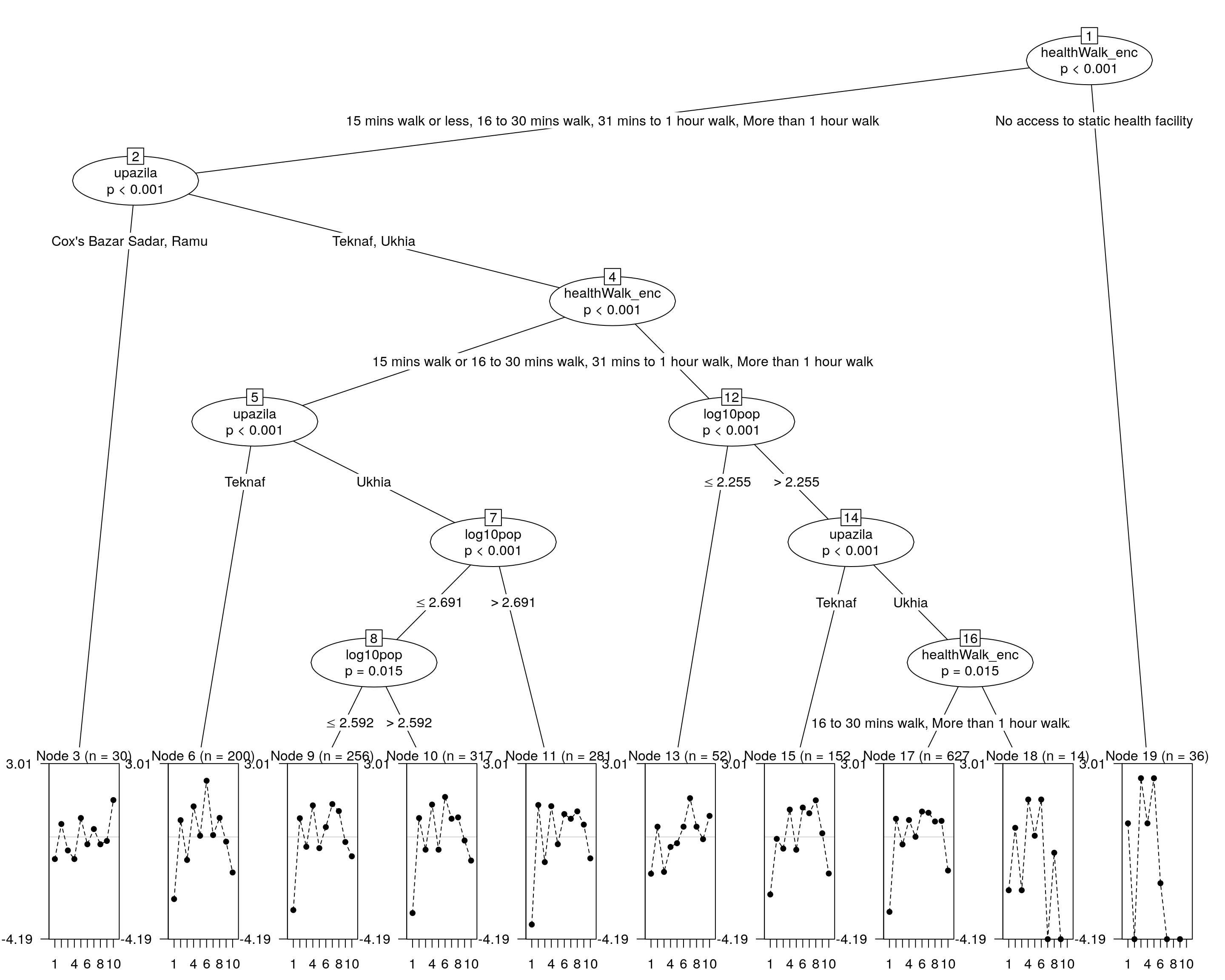
We can now extract the groups and descriptions.
## Compute the rashtree

kable(as.data.frame(itempar(raschtree)))| respl_fuel | respl_education | respl_food | respl_healthcare | respl_jobs | respl_nfis | respl_safety | respl_sanitation | respl_shelter | respl_water | |
|---|---|---|---|---|---|---|---|---|---|---|
| 3 | -0.9081861 | 0.5297518 | -0.5548941 | -0.9081861 | 0.7762540 | -0.3023904 | 0.3228189 | -0.3023904 | -0.1656218 | 1.5128443 |
| 6 | -2.5504606 | 0.6877839 | -0.9459138 | 1.2537563 | 0.0479739 | 2.3062634 | 0.0746899 | 0.7803303 | -0.1944528 | -1.4599705 |
| 9 | -3.0026343 | 0.7659191 | -0.4038798 | 1.2941211 | -0.4606402 | 0.4042383 | 1.3474463 | 1.0606580 | -0.2085509 | -0.7966776 |
| 10 | -3.1250880 | 0.7742496 | -0.5240226 | 1.3287548 | -0.5240184 | 1.6405011 | 0.7472167 | 0.8019314 | -0.1480432 | -0.9714814 |
| 11 | -3.5968421 | 1.3106673 | -1.0336702 | 1.2624465 | -0.3000406 | 0.9384069 | 0.7453142 | 1.0490368 | 0.5053854 | -0.8807043 |
| 13 | -1.5111376 | 0.4193461 | -1.4367589 | -0.4108577 | -0.2586516 | 0.4193461 | 1.5902196 | 0.4193461 | -0.0932484 | 0.8623964 |
| 15 | -2.3620951 | -0.0799298 | -0.4793960 | 1.1217560 | -0.5267838 | 1.2052988 | 0.9715678 | 1.5033119 | 0.1482659 | -1.5019957 |
| 17 | -3.0771201 | 0.7448512 | -0.3089609 | 0.6938837 | 0.0052486 | 1.0407114 | 0.9910606 | 0.6331558 | 0.6570708 | -1.3799010 |
| 18 | -2.1892234 | 0.3722365 | -2.1892233 | 1.5358228 | 0.0477570 | 1.5358228 | -Inf | -0.6490151 | -Inf | NA |
| 19 | 0.5575216 | -Inf | 2.4097182 | 0.5575217 | 2.4097182 | -1.8998867 | -Inf | NA | -Inf | NA |
We can also explore trees by focusing on one aspect…
## and plotting it...
plot(raschtree(resp ~ upazila, data = covariate), main = "For upazila")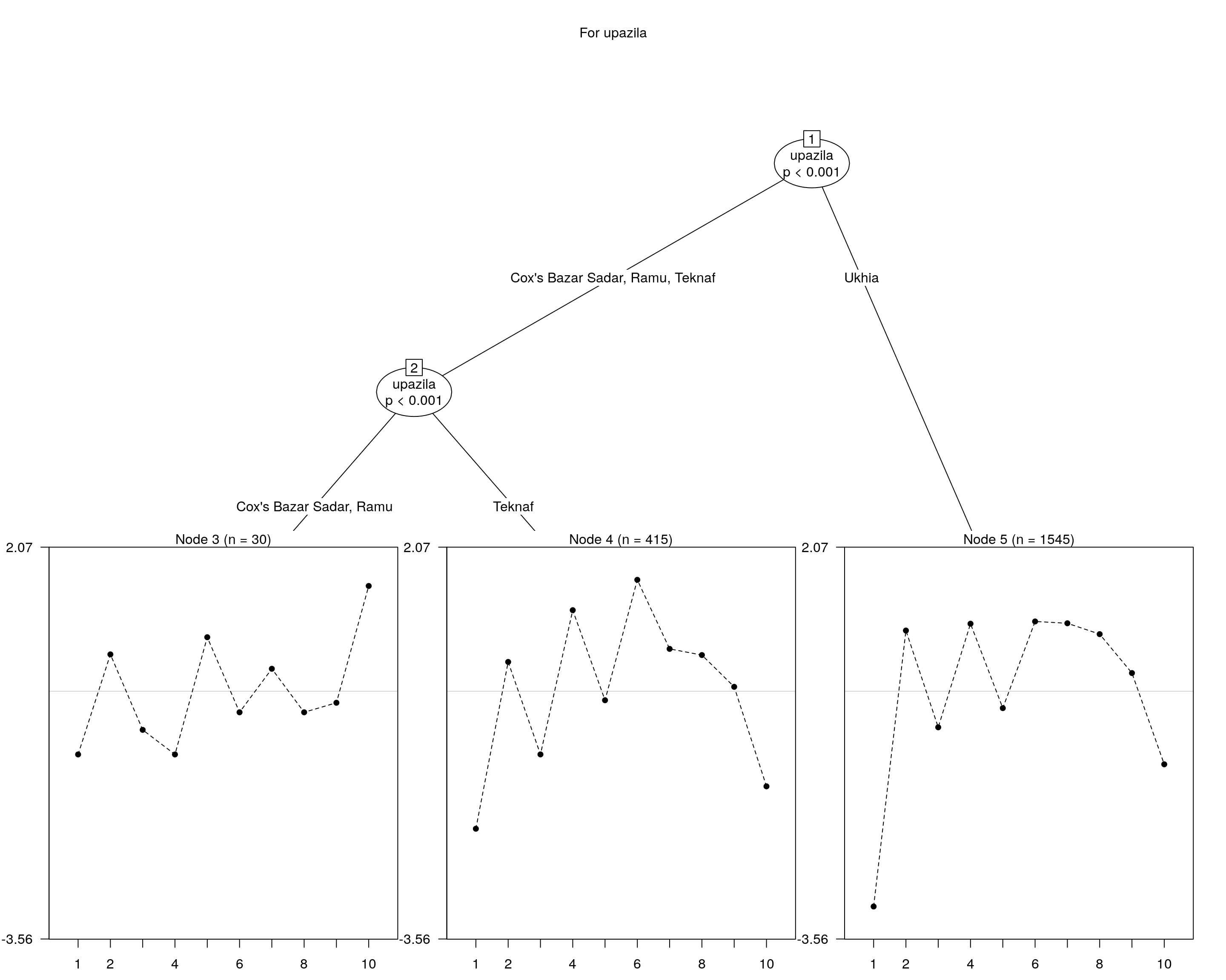
## and plotting it...
plot(raschtree(resp ~ log10pop, data = covariate), main = "For population")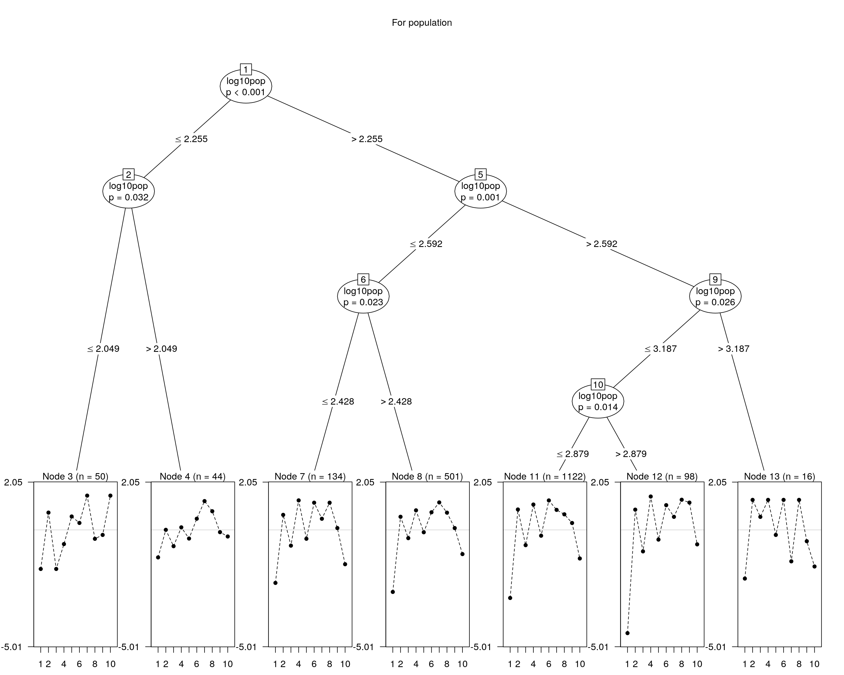
## and plotting it...
plot(raschtree(resp ~ healthWalk_enc, data = covariate), main = "For distance to Health Center")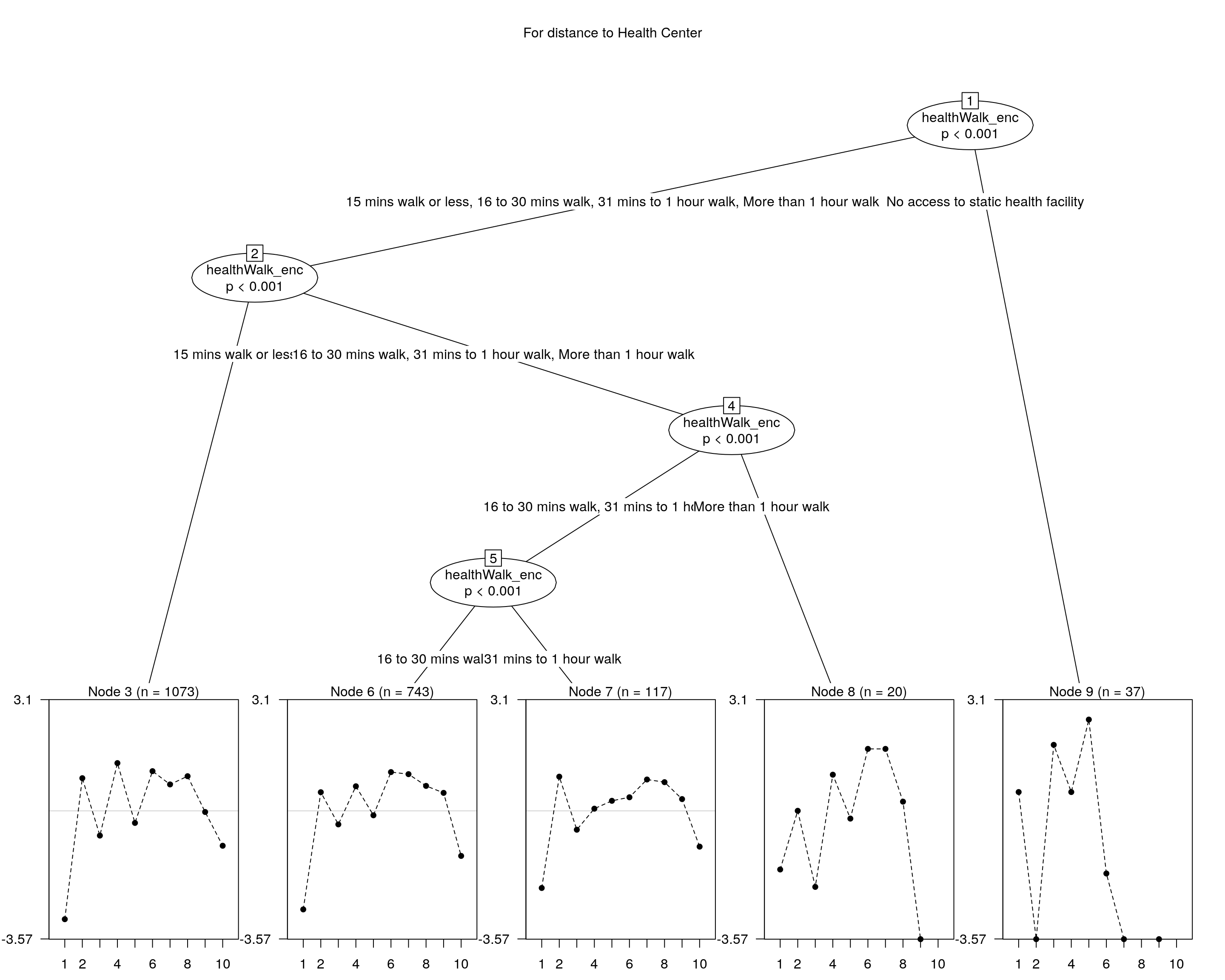
Share this post
Twitter
Google+
Facebook
Reddit
LinkedIn
StumbleUpon
Pinterest
Email